Sensor Fusion: Approach

This chapter describes how Aetherion will estimate the state of a flight vehicle from IMU, GNSS and barometer measurements: how the work is split with the Hemerion flight software, the filter form, the navigation frame, how the error state is built, and how the filter will be validated against truth. It records decisions as they are taken. Where a decision is still open, both options are given with their consequences.

Note

Status (v0.17.3). Step 2 (block scheme, vehicle configuration, log contract) is implemented in Aetherion/Estimation/Blocks.h, Configuration.h and LogContract.h. Step 5 is complete: SE23.h (the group), LciFrame.h (the navigation frame and gravity), EstimationState.h (state, retract and error in both conventions), ProcessModel.h (strapdown propagation, error dynamics, discrete transition) and MeasurementModels.h (GNSS position and velocity, barometer, with their innovation Jacobians in both conventions). Of step 6, EKF.h – the reference invariant EKF, InvariantEKF<S, C>, Joseph form, NEES/NIS – and the replay harness (Replay/, EkfReplay) are in and validated on an analytic truth and on synthetic logs in Hemerion’s formats, and the first real Hemerion log sets (check case 11, calm and in turbulence) replay consistently once Hemerion’s GPS epoch stamp is corrected. The working plan is TODO-sensor-fusion.md at the repository root.

Scope and ownership 

Sensor fusion is split between two repositories.

	Aetherion (MIT)	Hemerion (GPL-3.0)
Owns	Truth (plant FMUs, environment), estimator mathematics: state blocks, process and measurement models, a double-precision reference filter, the code generator, consistency analysis.	Everything a sensor touches: sensor FMUs (GPS, IMU, BMP390, MMC5983MA, radar altimeter), drivers, arrival time-stamping, the flight computer, co-simulation hosts.
Produces	Generated plain C for \(f\), \(h\) and their Jacobians, a configuration header, golden test vectors.	Co-simulation logs: decoded sensor samples and plant truth.

Dependency direction. Aetherion never depends on Hemerion. It replays the logs that Hemerion’s co-simulation hosts write. Generated code flows from Aetherion to Hemerion; sensor code never flows back. This keeps the licences compatible and means the estimator can be developed and validated without the flight software in the build.

Steps. The work is ordered in numbered steps shared by both repositories’ TODO files:

Step	Repository	Content
2	Aetherion	Block scheme, vehicle configuration, configuration hash, log contract.
3, 4	Hemerion	Sensor FMUs publish realised bias values; filter rates.
5	Aetherion	Process and measurement models, scalar-templated and AD-friendly.
6	Aetherion	Reference EKF (double precision), replay harness, time base, delayed GNSS measurements, NEES/NIS.
7, 7b	Aetherion	Tuning and observability on the check cases; float32 and covariance form.
8	Aetherion	Code generation (CppADCodeGen) and golden vectors.
9	Hemerion	Replay equivalence of the embedded filter against the golden vectors.

Filter form 

The estimator is an invariant extended Kalman filter (IEKF) [BB17, BB18] on the group of extended poses, with Euclidean bias states appended.

State space 

The navigation core is one element of \(\SE_2(3)\), the group of extended poses (rotation plus two vectors) [Bar17]:

\[\begin{split}X = \begin{bmatrix} R & v & p \\ 0_{1\times 3} & 1 & 0 \\ 0_{1\times 3} & 0 & 1 \end{bmatrix}, \qquad R \in \SO(3),\quad v, p \in \R^3,\end{split}\]

with \(R \equiv {}^{L}\!R_{B}\) the attitude (body \(B\) to navigation frame \(L\), see Navigation frame: launch-centred inertial), and \(v, p\) the inertial velocity and position resolved in \(L\). Composition is matrix multiplication,

\[X_1 X_2 = (R_1 R_2,\; R_1 v_2 + v_1,\; R_1 p_2 + p_1).\]

The group has dimension 9. A tangent vector is \(\xi = (\phi, \nu, \rho) \in \R^9\), with hat map

\[\begin{split}\xi^\wedge = \begin{bmatrix} [\phi]_\times & \nu & \rho \\ 0_{2\times 3} & 0 & 0 \end{bmatrix}.\end{split}\]

The exponential map has a closed form built from the \(\SO(3)\) exponential and left Jacobian \(J_l(\phi)\),

\[\Exp(\xi) = \big(\Exp(\phi),\; J_l(\phi)\,\nu,\; J_l(\phi)\,\rho\big),\]

so it reuses ODE/RKMK/Lie/SO3.h (see Group Exponential and Logarithm for the \(\SE(3)\) case). The inverse and, away from the \(\SO(3)\) cut locus, the logarithm are

\[X^{-1} = \big(R^{\mathsf T},\; -R^{\mathsf T} v,\; -R^{\mathsf T} p\big), \qquad \Log(X) = \big(\phi,\; J_l(\phi)^{-1} v,\; J_l(\phi)^{-1} p\big), \quad \phi = \Log(R).\]

The tangent coordinates \(\nu, \rho\) are not the physical differences \(v - \hat v\), \(p - \hat p\); how they relate depends on the error convention (below). The column order \((R, v, p)\) follows SE23.h; some of the literature swaps \(v\) and \(p\), which permutes every block matrix below.

The full state is \(\SE_2(3) \times \R^7\): the navigation core plus a gyro bias \(b_g \in \R^3\), an accelerometer bias \(b_a \in \R^3\) and a barometer bias \(b_p \in \R\).

Kinematics and the group-affine property 

With \(\tilde\omega, \tilde a\) the gyro and accelerometer readings, the strapdown kinematics in the inertial frame \(L\) are

\[\dot R = R\,[\tilde\omega - b_g]_\times, \qquad \dot v = R\,(\tilde a - b_a) + g_L(p), \qquad \dot p = v, \qquad \dot b_g = w_g,\quad \dot b_a = w_a,\quad \dot b_p = w_p,\]

(white noise on the readings omitted). A system \(\dot X = f_u(X)\) is group-affine [BB17] if, for all \(X_1, X_2\),

\[f_u(X_1 X_2) = f_u(X_1)\,X_2 + X_1\,f_u(X_2) - X_1\,f_u(I)\,X_2 .\]

For constant gravity the navigation kinematics above are group-affine. The consequence is that the left- and right-invariant errors defined below obey dynamics that do not depend on the state estimate. The linearisation is then exact for the navigation error, a poor initial attitude does not corrupt the propagation Jacobian, and in the deterministic setting the filter is a locally stable observer [BB17].

Two things break the property in this filter, both mildly:

Gravity varies with position. \(g_L(p)\) is evaluated with the WGS-84 model (Navigation frame: launch-centred inertial). Its gradient \(G = \partial g_L / \partial p\) is of order \(\mu / r^3 \approx 1.5\times 10^{-6}\,\mathrm{s^{-2}}\) (the square of the Schuler frequency). It adds an estimate-dependent term that is negligible over flights of minutes: a 100 m position error gives about \(10^{-4}\,\mathrm{m/s^2}\).
Biases. Bias states do not fit the group structure. They are kept as Euclidean states (the “imperfect IEKF” of [HGEG20]), and their coupling into the navigation error is where the two error conventions differ (below).

Error convention (open)

Important

Not yet decided, and deliberately not blocking. Step 5 is written with the convention as a template parameter of the process and measurement models, so both filters exist from the first commit and the decision is taken on evidence (Evidence: Monte Carlo prototype), not in advance. The configuration descriptor of step 2 names the convention, so each choice has its own configuration hash; the implementation currently carries right-invariant as a provisional value. Only the configuration that is generated for the flight computer (step 8) has to commit to one.

The two candidate errors on the navigation core, with \(\hat X\) the estimate and \(\zeta = b - \hat b\) the bias error, are

\[\text{right-invariant:}\quad \eta_R = X \hat X^{-1} = \Exp(\xi), \qquad X \approx (I + \xi^\wedge)\,\hat X,\]

\[\text{left-invariant:}\quad \eta_L = \hat X^{-1} X = \Exp(\xi), \qquad X \approx \hat X\,(I + \xi^\wedge).\]

To first order, the right-invariant components are world-frame quantities, \(v - \hat v = \nu + [\phi]_\times \hat v\) (and likewise for \(p\)). The left-invariant ones are body-frame quantities, \(v - \hat v = \hat R\,\nu\).

Propagation. With \(\hat\omega = \tilde\omega - \hat b_g\) and \(\hat a = \tilde a - \hat b_a\), and constant gravity:

\[\begin{split}\text{RI:}\quad \dot\xi = \underbrace{\begin{bmatrix} 0 & 0 & 0 \\ [g]_\times & 0 & 0 \\ 0 & I & 0 \end{bmatrix}}_{A_R}\xi \;-\; \Ad_{\hat X} \begin{bmatrix} \zeta_g \\ \zeta_a \\ 0 \end{bmatrix}, \qquad \Ad_{\hat X} = \begin{bmatrix} \hat R & 0 & 0 \\ [\hat v]_\times \hat R & \hat R & 0 \\ [\hat p]_\times \hat R & 0 & \hat R \end{bmatrix},\end{split}\]

\[\begin{split}\text{LI:}\quad \dot\xi = \underbrace{\begin{bmatrix} -[\hat\omega]_\times & 0 & 0 \\ -[\hat a]_\times & -[\hat\omega]_\times & 0 \\ 0 & I & -[\hat\omega]_\times \end{bmatrix}}_{A_L(\hat\omega,\,\hat a)}\xi \;-\; \begin{bmatrix} \zeta_g \\ \zeta_a \\ 0 \end{bmatrix}.\end{split}\]

In the RI form the navigation block is constant, but the bias coupling and the process noise (\(\Ad_{\hat X}\, Q\, \Ad_{\hat X}^{\mathsf T}\)) depend on the estimate. In the LI form the navigation block depends on the IMU readings, but not on the estimate, and the bias coupling is constant.

Measurements. A GNSS position fix is \(Y = p + V\); in the group’s terms, \(Y = X b\) with \(b = (0, 0, 1)\), which [BB17] calls a left-invariant observation. GNSS velocity is the same with \(b = (0, 1, 0)\). A magnetometer reading \(Y = R^{\mathsf T} m\) is a right-invariant observation, \(Y = X^{-1} b\). The innovation Jacobians on the navigation core are:

Measurement	RI: \(H\) on \((\phi, \nu, \rho)\)	LI: \(H\) on \((\phi, \nu, \rho)\)
GNSS position	\([\,-[\hat p]_\times,\; 0,\; I\,]\)	\([\,0,\; 0,\; I\,]\), innovation \(\hat R^{\mathsf T}(Y - \hat p)\)
GNSS velocity	\([\,-[\hat v]_\times,\; I,\; 0\,]\)	\([\,0,\; I,\; 0\,]\), innovation \(\hat R^{\mathsf T}(Y - \hat v)\)
Barometer \(h(p) + b_p\)	\(\nabla h^{\mathsf T}[\,-[\hat p]_\times,\; 0,\; I\,]\)	\(\nabla h^{\mathsf T}[\,0,\; 0,\; \hat R\,]\)
Magnetometer (deferred)	\([\,[m]_\times,\; 0,\; 0\,]\), innovation \(\hat R Y - m\)	\([\,[\hat R^{\mathsf T} m]_\times,\; 0,\; 0\,]\)

Each pairing (world-frame measurement with LI, body-frame measurement with RI) gives a constant Jacobian; the other pairing gives one that depends on the estimate. The barometer is a nonlinear function of position and depends on the estimate either way.

Trade-off for this filter.

	Right-invariant	Left-invariant
Navigation error dynamics	Constant (gravity only)	IMU-dependent, estimate-independent
Bias coupling	\(-\Ad_{\hat X}\), estimate-dependent	\(-I\), constant
GNSS position / velocity \(H\)	Estimate-dependent	Constant
Magnetometer \(H\) (later)	Constant	Estimate-dependent
Size of the coupling terms in LCI	\([\hat p]_\times\) with \(\lVert\hat p\rVert\) up to \(\sim 10^5\) m: 1 mrad of \(\phi\) maps to \(\sim 100\) m in \(\rho\)	Bounded by \(\lVert\hat R\rVert = 1\)

The first configuration is updated by world-frame measurements only (GNSS position, GNSS velocity, barometric altitude) and carries biases, which points to LI on structural grounds. The RI form keeps the navigation block constant and anticipates the magnetometer. The structural arguments do not settle the question, so it is settled on evidence (below).

First-order equivalence 

The two errors are related exactly by the adjoint of the estimate, \(\eta_R = \hat X \eta_L \hat X^{-1}\), so \(\xi_R = \Ad_{\hat X}\,\xi_L\) and \(P_R = \Ad_{\hat X} P_L \Ad_{\hat X}^{\mathsf T}\). Pushing this map through every step of the filter: the propagation matrices, the bias couplings and the process noise map onto each other exactly, and so do the measurement Jacobians (\(H_R \Ad_{\hat X} = H_L\), up to the rotation of the innovation by \(\hat R^{\mathsf T}\)), the gains and the corrected state (because \(\hat X \Exp(\xi) \hat X^{-1} = \Exp(\Ad_{\hat X}\xi)\)). The one place they differ is after an update: the estimate jumps from \(\hat X^-\) to \(\hat X^+\), each filter keeps its covariance unchanged, and the two are then no longer related by \(\Ad_{\hat X^+}\) but differ by about \(\Ad_{\Exp(\delta)} \approx I + \ad_\delta\). The difference is second order in the correction \(\delta\): negligible for small corrections, decisive for large ones.

So the conventions differ in two respects only: behaviour under large corrections (initial heading error, onset of heading observability, reacquisition after an outage) and numerics (the coordinates the covariance is stored in).

Evidence: Monte Carlo prototype 

scripts/iekf_convention_mc.py is a NumPy prototype of the first configuration with the convention as a switch. Both conventions see the same truth, the same sensor samples and the same initial error (paired runs), so every difference is the convention’s.

Model. LCI frame, point-mass gravity with its gradient, MEMS-class IMU (gyro 5·10⁻⁵ rad/s/√Hz, accelerometer 7·10⁻⁴ m/s²/√Hz, random-walk biases), GNSS position (1.5 m horizontal, 3 m vertical) and velocity (0.1 m/s) at 5 Hz, barometric height with random-walk bias at 10 Hz, IMU at 50 Hz. Truth is an F-16-like flight at 250 m/s: 30 s straight, then S-turns up to about 35° of bank, with light turbulence; or straight throughout. Initial covariance is given in physical coordinates and mapped to each convention, so both start equivalent. Joseph-form update, no covariance reset after updates (standard IEKF practice).
Not modelled. Geodetic and ECEF mapping, latency, lever arm. These are the same for both conventions.
Verification. Every entry of \(F\) and \(H\) in both conventions was checked against central finite differences of the full nonlinear propagation and measurement functions. This check found that RI needs \(F\) averaged over the step: its bias coupling \(-\Ad_{\hat X}\) contains \([\hat p]_\times \hat R\), which changes within one IMU step at a rate of about \(\lVert\hat p\rVert \lVert\omega\rVert\), so a start-of-step \(F\) is only first-order accurate (an error of about \(\tfrac12\, dt\, \lVert\hat p\rVert \lVert\omega\rVert\) in that entry). LI is second-order either way, because the corresponding variation sits inside \(A_L\). With a trapezoidal \(F\) both match the finite differences to \(O(dt^2)\). This is an implementation requirement for step 5.

Results, 30 paired runs per scenario, 300 s each (--runs 30 --seed 1). ANEES is averaged over the last two thirds of the run (1 is consistent); “converged” is the median time after which the yaw error stays below 1°; “failed” counts runs whose covariance lost positive definiteness.

Scenario	Conv.	ANEES	Final yaw RMS [°]	Final pos. RMS [m]	Converged [s]	Failed
Nominal (yaw σ 2°)	LI / RI	1.06 / 1.00	0.052 / 0.052	0.31 / 0.31	30 / 30	0 / 0
Heading error 45°	LI / RI	20.1 / 1.26	0.058 / 0.051	0.32 / 0.31	77 / 37	0 / 0
Heading error 120°	LI / RI	2.8·10⁴ / 13.3	0.53 / 0.054	2.7 / 0.32	80 (2 never) / 48	0 / 0
GNSS outage 100–160 s	LI / RI	1.07 / 0.97	0.049 / 0.049	0.34 / 0.34	30 / 30	0 / 0
158 km out, straight, yaw σ 10°, float64	LI / RI	7.3 / 14.9	45 / 57	0.31 / 0.31	never / never	0 / 0
Same, float32 covariance	LI / RI	7.3 / 1.8·10¹⁴	45 / 80	0.31 / 5.4·10⁴	never / never	0 / 30
Nominal, float32 covariance	LI / RI	1.06 / 7.5·10⁸	0.052 / 48	0.31 / 300	30 / never	0 / 30

During the outage the maximum position error was 59 m (LI) and 51 m (RI); ANEES in the 20 s after reacquisition was 1.06 and 0.96.

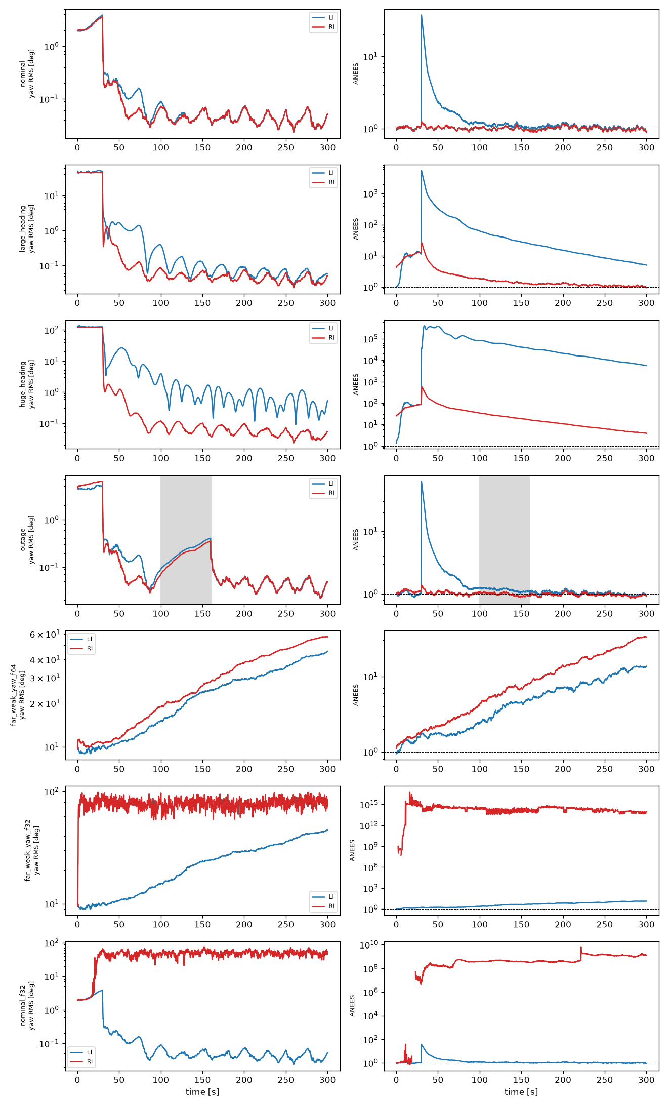
Yaw RMS and ANEES against time for LI and RI in seven scenarios — Yaw RMS (left) and ANEES (right) against time, LI blue, RI red; grey band is the GNSS outage.

Findings.

Equivalent in normal operation, as the first-order argument predicts: same final accuracy, same behaviour through a 60 s GNSS outage and at reacquisition.
RI handles large corrections better. With 45° and 120° of initial heading error RI converges about twice as fast and stays close to consistent. LI becomes badly overconfident when heading first becomes observable, and with 120° two LI runs never converge. The effect is visible even in the nominal case: at the first turn (t = 30 s), when heading becomes observable, LI’s ANEES spikes to about 30 and takes some 70 s to recover, while RI stays at 1.
LI is robust in float32; RI is not. With a plain Joseph-form covariance in float32, RI loses positive definiteness in every run: at the first update when 158 km from the origin, and within 3–10 s (at \(\lVert\hat p\rVert\) of 1–2.5 km) in the nominal case, after which the estimate diverges. LI in float32 reproduces its float64 results to every printed digit. This confirms the conditioning argument above: RI stores world-frame coordinates coupled through \([\hat p]_\times\) and \([\hat v]_\times\).
Long unobservable yaw: both overconfident. In 300 s of straight flight, yaw and the vertical gyro bias are unobservable and the yaw error grows to about 50°. Both filters become overconfident, RI more so (ANEES 14.9 against 7.3).

Caveats. One trajectory family and one sensor grade; no covariance reset after updates; float32 tested only with the Joseph form. A covariance reset (re-anchoring \(P\) with \(\Ad_{\Exp(\delta)}\) or the corresponding Jacobian after each update) acts exactly on the second-order term where the conventions differ, and may narrow finding 2. A UD or square-root covariance may rescue RI in float32 (finding 3). Both are the next experiments.

Implications. The evidence does not pick a single winner. It frames the decision as robustness to large heading errors (RI) against single-precision robustness (LI):

Without a magnetometer, initial heading is the hard part of the first configuration outside simulation, which favours RI.
If the flight computer runs the filter in float32, RI needs a square-root or UD covariance at least, and that is unproven; LI works with the Joseph form.
Remaining experiments, in order: covariance reset in both conventions; RI with UD / square-root covariance in float32; a sweep of initial heading error (5°, 10°, 20°) to find where LI stops being consistent, since a heading initialiser only needs to beat that bound; a second trajectory family (the rocket ascent).

Step 5 keeps both conventions behind the template parameter until these are done.

Implementation (step 5)

Aetherion/Estimation/ProcessModel.h implements the model above with the convention as a template parameter of errorJacobians<C>() and step<C>(), and EstimationState.h the matching retract<C>() / error<C>() pair (\(X \leftarrow \Exp(\delta)\hat X\) or \(\hat X \Exp(\delta)\); \(\xi = \Log(X\hat X^{-1})\) or \(\Log(\hat X^{-1}X)\)). Gravity is evaluated at the estimated position in the LCI frame (LciFrame.h, WGS-84 central + J2); its gradient enters the error dynamics with the central term only. The discrete transition is \(\Phi = I + \bar F\,dt + \tfrac12(\bar F\,dt)^2\) with \(\bar F\) the average of \(F\) at the start and the end of the step, as the prototype required.

The C++ repeats the prototype’s finite-difference check in tests/Estimation/test_ProcessModel.cpp, as a convergence test rather than a tolerance: the analytic \(\Phi\) and the linearisation of the nonlinear step are both second-order one-step maps, so their difference must fall by \(2^3\) when \(dt\) is halved. It does (7.9 RI, 7.4 LI), and with a start-of-step \(F\) the RI ratio is 4.00 – the first-order error described above. The same test caught a first-order inconsistency in the nonlinear step itself: rotating the specific force by the start-of-step attitude gives a map whose linearisation has no \(\partial v/\partial b_g\) term, while \(\Phi\) carries \(\tfrac12 dt^2 [a]_\times\) there. The propagation therefore rotates the velocity increment by the mid-step attitude \(\hat R\,\Exp(\omega\,dt/2)\). Finally, the same map is differentiated by CppAD through Eigen and the CondExp branches of \(\Exp\) and \(\Log\) and agrees with the finite differences to \(10^{-9}\) (RI) and \(10^{-7}\) (LI): the path the code generator takes is exercised now, not in step 8.

Propagation accuracy (open)

The step above is a second-order scheme. It is not the exact solution for constant inputs, and it does not use the RKMK integrators of RKMK Numerical Integration on Product Manifolds. Two alternatives are on record for a later comparison; neither is implemented in the estimator.

Exact constant-input step. With \(\omega, a\) (bias-corrected) and gravity \(g\) held constant over a step of length \(h\), and \(\phi = \omega h\), the kinematics integrate in closed form (the same structure underlies IMU preintegration on \(\SE_2(3)\) [BB20]):

\[R^+ = R\,\Exp(\phi), \qquad v^+ = v + g h + R\,h\,J_l(\phi)\,a, \qquad p^+ = p + v h + \tfrac12 g h^2 + R\,h^2 J_2(\phi)\,a,\]

\[J_2(\phi) = \int_0^1 (1-s)\,\Exp(s\phi)\,ds = \tfrac12 I + \tfrac16 [\phi]_\times + \tfrac1{24} [\phi]_\times^2 + \cdots .\]

\(J_2\) is not \(J_l\). The step is exact only under its assumptions: inputs held constant over the interval, and constant gravity. With position-dependent gravity and the replay’s averaged readings it is another approximation, if a better one in fast rotation.

RKMK [MK98]. Written as \(\dot X = X\,u(t, X)^\wedge\) with the body-trivialised field

\[u(t, X) = \big(\omega,\; a + R^{\mathsf T} g_L(p),\; R^{\mathsf T} v\big),\]

and \(X(t) = X_n \Exp(\Omega(t))\), the local coordinates obey \(\dot\Omega = \dexp^{-1}_{-\Omega}\big(u(t, X_n\Exp(\Omega))\big)\) with \(\dexp^{-1}_{-\Omega} u = u + \tfrac12[\Omega, u] + \tfrac1{12}[\Omega,[\Omega, u]] + \cdots\) (the sign is the one fixed in RKMK Numerical Integration on Product Manifolds; the opposite sign passes the usual tests and caps the order at two). The bracket on \(\Lie{se}_2(3)\), for \(\xi = (\phi, \nu, \rho)\) and \(\eta = (\psi, \mu, \sigma)\), is

\[[\xi, \eta] = \big(\phi\times\psi,\; \phi\times\mu - \psi\times\nu,\; \phi\times\sigma - \psi\times\rho\big).\]

A fourth-order state step is not a fourth-order filter: \(\Phi\) and \(Q_d\) would have to be made consistent with it, by the same convergence test as above. A fair comparison runs the present step, the exact constant-input step and RKMK4 on the same input reconstruction, and compares NEES/NIS and cost as well as state error. RKMK4 cannot beat the exact step when the inputs really are constant over each interval.

Navigation frame: launch-centred inertial 

Definition 

The navigation frame \(L\) is launch-centred inertial (LCI). Its origin is the launch or take-off point and its axes are the local NED axes at the initial time \(t_0\), frozen in inertial space from then on (they do not rotate with the Earth). With \(W\) the ECI frame, \(E\) ECEF and \(N\) local NED (notation of Coordinate Frames and Basic Notation and Launch-Site Initialization and Frame Chain):

\[r_{W,0} = {}^{W}\!R_{E}(t_0)\, r_E(\varphi_0, \lambda_0, h_0), \qquad {}^{W}\!R_{L} = {}^{W}\!R_{E}(t_0)\; {}^{E}\!R_{N}(\varphi_0, \lambda_0),\]

\[p = {}^{L}\!R_{W}\,\big(r_W - r_{W,0}\big), \qquad v = {}^{L}\!R_{W}\,\dot r_W, \qquad g_L(p) = {}^{L}\!R_{W}\; g_W\!\big(r_{W,0} + {}^{W}\!R_{L}\, p\big).\]

\(L\) differs from ECI by a constant rotation and translation, so it is inertial. The origin \((\varphi_0, \lambda_0, h_0)\) is read from the run-configuration sidecar of the replayed log (lat0_deg, lon0_deg, alt0_ft).

Why not local NED or ECEF 

Local NED about a fixed origin, with Earth rate neglected, is exactly group-affine under its own model. But Aetherion’s truth runs in ECI and the IMU measures inertial rates and specific force, so that model is wrong by:

Earth rate, \(15^\circ/\mathrm{h}\). It rotates with attitude in the body frame, so the gyro bias state cannot absorb it; over 10 min of weakly observable yaw this is about \(2.5^\circ\).
Coriolis, \(2\,\omega_\oplus \times v\): about 3.6 mg at 250 m/s, the size of a MEMS accelerometer bias.
Gravity direction: at distance \(d\) from the origin the local vertical is tilted by \(d/R_\oplus\) (\(0.45^\circ\) at 50 km), which the filter would read as tilt error.

It also cannot carry the rocket to orbit.

ECEF loses the group-affine property. Applying the test above to the ECEF strapdown model (Earth rate, Coriolis, centrifugal) with \(\Omega = -[\omega_\oplus]_\times\), the rotation and position rows pass, but the velocity row leaves the residual

\[(\Omega R_1 - R_1 \Omega)\,(v_2 + \Omega\, p_2) \neq 0 .\]

ECEF (or ECI) positions are also about \(6.4\times 10^6\) m, which float32 resolves to only about 0.5 m, the same as one 500 Hz integration step at 250 m/s.

In LCI there are no Earth-rate or Coriolis terms, the only violation of the group-affine property is the gravity gradient, truth and IMU are compared like with like, the same frame serves the rocket, and positions stay around \(10^5\) m (float32 resolution of a few centimetres).

Costs 

Gravity is evaluated at the estimated position, not taken as constant.
GNSS measurements are mapped through the time-dependent rotation \({}^{W}\!R_{E}(t)\):

\[Y_p = {}^{L}\!R_{W}\big({}^{W}\!R_{E}(t)\, r_E(\varphi, \lambda, h) - r_{W,0}\big), \qquad Y_v = {}^{L}\!R_{W}\; {}^{W}\!R_{E}(t)\, \big({}^{E}\!R_{N}(\varphi,\lambda)\, v_{N} + \omega_\oplus \times r_E\big).\]

GNSS velocity is Earth-relative; the transport term \(\omega_\oplus \times r_E\) (up to 465 m/s) makes it inertial.
Time base. A timing error \(\delta t\) rotates the ECEF-to-LCI mapping by \(\omega_\oplus\,\delta t\), about 0.47 m per millisecond at the Earth’s radius. The replay time-base calibration (step 6) must leave a residual well below 1 ms.
Heading and yaw covariance are reported by rotating into the current local NED frame.

Error-state composition 

Blocks 

The error state is composed from named blocks, each with a fixed dimension, units, frame and process model (Aetherion/Estimation/Blocks.h):

Block	Dim	Units	Frame	Process model	Rank
`nav_core`	9	rad, m/s, m (\(\phi, \nu, \rho\))	LCI	strapdown	0
`gyro_bias`	3	rad/s	body	random walk	1
`accel_bias`	3	m/s²	body	random walk	2
`baro_bias`	1	m of pressure altitude	–	random walk	3

The block’s position in the error vector is fixed by its rank, never by the order a configuration lists blocks, so the navigation core is always first and two configurations that share a block agree on its layout. The barometer bias is a random walk, not a constant: a temperature offset gives a pressure-altitude error that grows with height, so the bias drifts in a climb.

Vehicle configuration 

A configuration (Configuration.h) selects blocks and measurements at build time. Each measurement declares the blocks it depends on, and a configuration that selects a measurement without its blocks is rejected. Whether a measurement is available at run time (no GNSS fix, barometer below its rated floor) is handled by skipping updates, never by resizing the state.

The first configuration, kNavBaroGnss16, carries all four blocks (16 error states) and the updates GNSS position, GNSS velocity and barometer. It has no magnetometer (deferred until Hemerion’s replay equivalence, step 9, has passed once) and no GNSS antenna lever arm.

Configuration hash 

Every configuration has a canonical text descriptor and a 64-bit FNV-1a hash of it. The descriptor names the group, the error convention and the navigation frame, then the blocks in rank order and the measurements with their block dependencies:

aetherion.estimation/1
group=SE2(3)
error=right-invariant
frame=LCI
block=nav_core,9,rad[3],m/s[3],m[3],LCI,strapdown
block=gyro_bias,3,rad/s[3],body,random_walk
block=accel_bias,3,m/s^2[3],body,random_walk
block=baro_bias,1,m[1],none,random_walk
meas=gnss_position,3,nav_core
meas=gnss_velocity,3,nav_core
meas=barometer,1,nav_core+baro_bias

(error=right-invariant is provisional; see the error convention above.) Generated code and golden vectors carry the hash, so the flight software can reject a mismatch. The hash of the first configuration is pinned in tests/Estimation/test_Configuration.cpp: changing a block, a measurement or the filter form fails that test until the pin is updated together with the generated artefacts.

Measurement models 

Measurement models (step 5) are written against what Hemerion’s drivers decode, not against idealised quantities:

GNSS position from UBX-NAV-PVT latitude, longitude and height. The height is ellipsoidal (NAV-PVT height), mapped to LCI as above.
GNSS velocity from UBX-NAV-PVT velN, velE, velD, made inertial and mapped to LCI as above.
Barometer: compensated pressure converted to pressure altitude by inverting the standard atmosphere, modelled as \(y = h(p) + b_p + v\). Constant offsets between pressure altitude and ellipsoidal height (geoid, non-standard sea-level pressure) are absorbed by \(b_p\).

The first configuration assumes the GNSS antenna is at the IMU (no lever arm). The models are scalar-templated, in the same style as the dynamics, so one definition serves the double-precision reference filter (via CppAD Jacobians, [Bel25]) and the code generator.

Implementation (step 5). Aetherion/Estimation/MeasurementModels.h provides the raw-to-LCI mappings (gnssPositionLci, gnssVelocityLci with the transport term, nedToLci for the receiver’s NED accuracies, all through the Earth rotation angle at the fix’s time, LciFrame::earthRotationAngle), the pressure-altitude inversion pressureAltitude_m (the exact layer-by-layer inverse of US1976Atmosphere, including the geopotential conversion and the above-ceiling decay), and the linearised updates gnssPosition<C>, gnssVelocity<C>, barometer<C> returning innovation, Jacobian and the measurement covariance in the convention’s innovation coordinates (rotated by \(\hat R^{\mathsf T}\) for LI). The barometer’s height is Environment::GeometricAltitude_m of the estimated position (height above the ellipsoid to 0.1 m below 15 km), with an analytic gradient; the iterative ECEFToGeodeticWGS84 is not used because it is compiled for double only and cannot be taped. Every Jacobian is checked against central differences of the nonlinear maps in both conventions, and the barometer’s again through CppAD, in tests/Estimation/test_MeasurementModels.cpp.

Replay and log contract 

The reference filter runs on logs written by Hemerion’s co-simulation hosts. No new format is defined; the existing logs are the contract:

Log	Written by	Columns read
`gps_fixes.csv`	flight computer	`host_time_s`, `fix_type`, `latitude_deg`, `longitude_deg`, `altitude_m`, `horizontal_accuracy_m`, `vertical_accuracy_m`; for GNSS velocity `vel_north_mps`, `vel_east_mps`, `vel_down_mps`, `speed_accuracy_mps` (not yet written)
`imu_samples.csv`	flight computer	`part_time_s`, `host_time_s`, `accel_{x,y,z}_mps2`, `gyro_{x,y,z}_rad_s`
`baro_samples.csv`	flight computer	`part_time_s`, `host_time_s`, `pressure_pa`, `temperature_c`
truth CSV	co-simulation host	`time`, `out.{lat_deg, lon_deg, alt_m}`, `out.v_{north,east,down}_m_s`, `out.{yaw,pitch,roll}_rad`
`<truth>.config`	co-simulation host	`lat0_deg`, `lon0_deg`, `alt0_ft`, `gps_latency_s`, `realtime_factor`

LogContract.h binds columns by name when a log is opened and reports every missing column at once, so a rename on the Hemerion side fails loudly instead of silently shifting a column. Which columns are required depends on the configuration.

Time base. host_time_s is the flight computer’s clock and equals simulation time only when the host runs at a real-time factor of 1; part_time_s is the sensor’s own clock; the truth log’s time is simulation time. The replay harness maps flight-computer time onto simulation time with a fit over the IMU log, which carries both clocks. GNSS fixes arrive late (--gps-latency) and are handled as delayed measurements.

The harness (step 6). Aetherion/Estimation/Replay/ and the EkfReplay executable (src/Examples/EkfReplay):

Csv.h, Logs.h: the logs as typed records, columns bound by name through the contract; a log the configuration does not use is not required.
TimeBase.h: the least-squares line host = offset + scale * part over the IMU log, with its residual statistics, so a wrong clock assumption shows as a residual rather than a silent offset.
TruthState.h: the truth row (geodetic position, Earth-relative NED velocity, ZYX Euler angles) as an LCI state at era(t) = w_e t, and the inverse for reporting attitude errors in the local NED frame.
Replay.h: the loop. Each IMU interval is propagated with the readings held at the average of its two bounding samples; a measurement whose validity time falls inside an interval splits it – predict to that time, apply, predict the remainder. The clock conventions sit in one ReplayTiming struct, set from a survey of Hemerion’s writers (origin/main 7da6057, 2026-10-13): IMU samples on their part_time_s (simulation time unless the FMU’s clock skew and jitter are on); barometer samples on their part_time_s, which is the BMP390’s SENSORTIME register and wraps every 512 s, unwrapped against the fit-mapped host time; a fix at its nominal_time_s – the epoch in simulation time, index-based, so the GPS latency cancels in it (one fix period late in Hemerion 7da6057; see the first real replay below) – falling back to the mapped arrival time minus gps_latency_s if that column is absent. Epochs without a fix are written with empty fields and are skipped, as are fixes below 3D in Hemerion’s own fix_type enum (0 none, 1 2D, 2 3D – not UBX’s numbering). This is the replay reference, which may know the latency, while the flight filter must recover it from the arrival stamps (Hemerion step 10) and is judged against the reference by the golden vectors. Output: one row per IMU sample (estimate, truth, error in the filter’s coordinates, NEES, sigmas), one per update (NIS), and a summary. NEES is over the navigation core only until the sensor FMUs publish their realised biases (Hemerion step 3).

Other facts of the logs the harness relies on, from the same survey: the truth CSV is written by the host at one row per communication step (0.1 s for the trim host, 0.01 s for the autopilot host) and is interpolated; the IMU’s host_time_s is the arrival of the whole burst, so the time-base fit shows the step as a sawtooth residual and is a cross-check, not a clock; unpaced (realtime_factor 0) the polled barometer yields only a few dozen conversions per 200 s; the GPS FMU encodes the plant’s altitude as both height and hMSL (no geoid on either side) and velD as zero; the plant starts at Earth rotation angle zero at t = 0 and Hemerion sets no epoch.

Validated on synthetic logs written in Hemerion’s formats from the manoeuvring analytic truth (tests/Estimation/test_Replay.cpp): the time base is recovered to the stamping jitter, and both conventions are consistent at the GNSS floor. Over 20 noise seeds (120 s each, second half; the test pins seed 3) the two are indistinguishable: ANEES of the navigation core 1.04 mean (0.44 to 2.04), NIS per dimension 0.91 to 1.13 for every measurement, position 0.34 m RMS, tilt 0.43° mean for both (0.05 to 1.24°), and neither convention has the lower tilt error in more than 11 of the 20 seeds. A single seed can suggest a convention preference: seed 3 gives 0.11° LI against 0.90° RI. Two things that test caught: applying a measurement “after the IMU step that reaches it” lets a fix stamped microseconds after a boundary wait a whole period, a mean lag of half an IMU period that at 120 m/s is a 0.6 m along-track bias rotating with the heading (ANEES 3.8 with every NIS at 1 – the signature of a truth/measurement disagreement rather than a filter fault); and holding the earlier IMU sample over the interval, rather than the average, reads as a bias.

First real replay (2026-10-14). Hemerion 7da6057, check case 11 for 200 s at --rtf 1, calm and in light-to-moderate turbulence (W20 = 8 m/s), replayed with nav-baro-gnss. As logged, the filter was ANEES ~1300 with GNSS NIS at 1 and 17 m position RMS: the truth/measurement-disagreement signature again. The fixes match the truth with no filter involved once moved 0.100 s earlier (to 1 cm along-track; 17.2 m at 172 m/s without the shift). Hemerion’s flight computer stamps fix_count * fix_period with fix_count counted from 1, while the GPS FMU encodes the plant state at the start of the co-simulation step, so nominal_time_s is one fix period late. With the stamps corrected:

Run	Conv.	ANEES	NIS GNSS	Position RMS	Tilt RMS	Yaw RMS
Case 11, calm	RI / LI	1.76 / 0.74	0.98	0.44 m	0.32° / 0.13°	23° / 9°
Case 11, turbulence	RI / LI	1.17 / 1.31	1.03	0.46 m	0.10° / 0.22°	4.1° / 4.8°

Yaw drifting in calm trimmed flight is the expected weak observability without a magnetometer; turbulence makes it observable. Barometer NIS is 0.11 in both runs, so the default 1 m pressure-altitude sigma is pessimistic (step 7). The IMU stamps are consistent, but its 100 Hz samples see the plant’s specific force and rates held over each 0.1 s communication step (best shift against truth −0.055 s in turbulence); the manoeuvring cases of step 7 should run at a 0.01 s step.

Known gaps. Hemerion’s GPS driver does not yet decode NAV-PVT velocity, so kNavBaroGnss16 does not bind against current GPS logs (a test asserts this). The rocket truth log carries no attitude, and the rocket plant publishes only Euler angles, which are singular at the 90° pitch of a vertical launch; the rocket configuration needs a quaternion truth output.

Reference filter (step 6)

Aetherion/Estimation/EKF.h is the reference filter, InvariantEKF<S, C>: predict() through ProcessModel::step<C>, updateGnssPosition(), updateGnssVelocity(), updateBarometer() through the measurement models, with the Joseph-form covariance update and the state corrected by retract<C>. A measurement the configuration does not carry is skipped and the result says so. The covariance lives in the convention’s error coordinates; covarianceFromPhysical() maps an initial covariance given in physical coordinates into them, so both conventions start equivalently. No covariance reset after updates, no delayed-measurement handling: the replay harness owns time.

tests/Estimation/test_EKF.cpp runs both conventions on an analytic truth – a level circle at 120 m/s with the bank swinging ±15° about the coordinated value and the pitch ±8° – with a MEMS-grade IMU, constant biases, GNSS position and velocity at 5 Hz, barometer at 10 Hz, from a start 5° off in heading, 1° in tilt, 20 m in position. After 240 s both are consistent (NEES 0.9 and 0.8 of 16 degrees of freedom, NIS 1.03 of 3 and 1.08 of 1), position is at the GNSS floor (0.15 m), tilt within 0.35°, and yaw – weakly observable without a magnetometer – is still coming down (0.9° RI, 0.4° LI). The first version of that truth, an unbanked turn, taught a lesson worth recording: with the attitude fixed relative to the specific-force vector, every tilt error is indistinguishable from a body-frame accelerometer bias, and the filter drifts along that direction with NEES growing while GNSS keeps position and velocity perfect. The check cases of step 7 bank in their turns; a synthetic truth must too.

Validation plan 

Consistency is judged against truth with the normalised estimation error squared (NEES) and the normalised innovation squared (NIS) [Sim06],

\[\mathrm{NEES} = e^{\mathsf T} P^{-1} e, \qquad \mathrm{NIS} = z^{\mathsf T} S^{-1} z,\]

with \(z\) the innovation and \(S = H P H^{\mathsf T} + R\) its covariance. For a consistent filter their expectations are the error and measurement dimensions. The error \(e\) must be taken in the convention’s own coordinates (x.error<C>(truth), as EKF.h does), because that is what \(P\) describes; a physical difference \(p - \hat p\) scored against an RI covariance is not a consistency test. Bias-state NEES needs the realised bias values, which the sensor FMUs will publish (Hemerion step 3).

Tuning and observability (step 7) use the F-16 check cases with turbulence on (in calm air every body rate on case 11 stays below one gyro count):

Case	Purpose
11	Baseline: position, velocity, tilt and bias consistency.
12	Degraded mode: no GNSS fix, barometer below its rated floor.
13.1	Barometer bias drift in the climb.
13.3, 13.4	Heading observability.

Without a magnetometer, yaw is only weakly observable in trimmed flight, so yaw covariance growing on case 11 is expected, not a bug. Heading is initialised from truth. It is not initialised or aided from GNSS course: in a 10 m/s crosswind, course and yaw differ by 2.28°.

Numerical form (step 7b). The reference filter is rerun in float32, and the covariance form (Joseph form, or UD / square-root) is chosen while truth is still available. The choice is an input to the embedded implementation. A UKF is run as a cross-check once the EKF is consistent.

Closed-loop use (planned)

Replay shows that the filter is consistent on a fixed record of inputs. It does not show that the vehicle stays acceptable when its controller flies on the estimate: in replay an estimation error cannot change the trajectory that produces the next measurement, and in flight it does. Both questions need answering; neither answers the other.

No commands in the navigation filter. The gyro and accelerometer measure the motion that every force and moment produces, control included, so the strapdown kinematics above need no actuator commands, and stay independent of aerodynamic derivatives and actuator models. Commands enter only through model aiding (below), never by replacing measured specific force with commanded acceleration.

One filter, three drivers. The same filter, driven by typed, timestamped events, runs in offline replay (reproducibility, Jacobians, NEES/NIS, regression), in closed-loop co-simulation with live sensor FMUs (stability, transients, dropout and reacquisition, scheduling) and on the flight computer (deadlines, numerics, fault response). Reading a CSV log is an adapter around the filter, not part of it; InvariantEKF already has this shape (predict, one update* per measurement, time owned by the caller).

Three times per measurement. A measurement has a validity time \(t_m\), an arrival time \(t_a\) and is used at a control epoch \(t_c\), normally \(t_m \le t_a \le t_c\). Applying a late GNSS fix as if it were current is a time-alignment error, and in LCI also a frame error through \({}^{W}\!R_{E}(t)\). The replay reference may apply the fix at \(t_m\) because it reads the whole log; the flight filter keeps a bounded history of state, covariance and IMU samples, corrects at \(t_m\) and repropagates to the present (Hemerion step 10). An estimate handed to the controller at \(t_c\) must never contain a measurement that had not arrived by \(t_c\), and any dead-reckoning past the last IMU sample is bounded and reported.

Controller-facing contract. At minimum: epoch, frame, state, covariance (or a bounded quality figure), age, and a health mode – uninitialised, aligning, nominal, degraded, invalid – each with defined control behaviour. A GNSS outage leaves attitude usable while position uncertainty grows; reacquisition can produce a large correction, which guidance must not see as an unbounded step in its reference.

Acceptance. Mean error and consistency are necessary but not sufficient. The closed-loop matrix varies initial yaw error, aerodynamic uncertainty, wind and turbulence, GNSS dropout and delay, computation overruns and manoeuvres, and judges tracking error, actuator activity and saturation, transients at large corrections, estimate age and missed deadlines, innovation consistency, and safe fallback. The two error conventions are compared on these too, not on position RMS alone: they differ precisely in how they behave under large corrections (Evidence: Monte Carlo prototype), and that is what a controller feels.

Model-aided estimation (deferred)

The navigation predictor is strapdown: IMU samples drive it, and the 6-DOF plant is not evaluated. Aetherion’s differentiable plant could add information in two ways, both deferred.

Plant aiding as a measurement. Keep the strapdown core and add the plant as an optional source,

\[z_{\mathrm{model}} = h_{\mathrm{model}}(X, b, u_c, \hat\theta) + \epsilon_{\mathrm{model}}, \qquad \operatorname{Cov}(\epsilon_{\mathrm{model}}) = R_{\mathrm{model}},\]

for example on air-relative velocity or a slowly varying parameter. \(R_{\mathrm{model}}\) must cover aerodynamic, actuator and wind uncertainty and the model’s validity envelope. If the model output was computed from an IMU sample or measurement the filter has already used, the errors are correlated, and treating them as independent makes the covariance overconfident: model the correlation, augment the state with the shared uncertainty, or leave the redundant information out. The inertial core stays common across vehicles while the aiding blocks change with the configuration (aerodynamics and air data for the fixed wing, variable mass and propulsion for the rocket, mode-dependent models for the tail-sitter).

Plant as the process model. The state then grows beyond \((R, v, p)\) to body rates, actuator or propulsion states and model parameters. CppAD gives \(A_z = \partial f/\partial z\) and \(B_u = \partial f/\partial u_c\) of the plant, but these are not the filter’s error Jacobian: that is the derivative of the discrete perturbed flow, mapped back through the retraction,

\[F_d = \frac{\partial}{\partial\xi}\, \mathcal R^{-1}_{\Phi_h(\hat z)}\!\Big( \Phi_h\big(\mathcal R_{\hat z}(\xi), u_c\big)\Big)\Big|_{\xi = 0},\]

which differs between \(\hat X\Exp(\xi)\) and \(\Exp(\xi)\hat X\) even for identical physics. Taping that map, not the continuous \(A_z\), is the AD route, and it is the same consistency requirement step 5 met for the strapdown step. Such a filter inherits every aerodynamic, thrust, actuator and wind modelling error, so it must be validated against a plant that is deliberately perturbed from the filter’s model, never only against itself.

Code generation 

The double-precision reference filter is the specification. For the flight computer, a host-side generator (CppADCodeGen, step 8) emits plain C for \(f\), \(h\) and their Jacobians for one configuration, together with a header that carries the dimension, block offsets and configuration hash. Golden vectors (recorded inputs and outputs of the reference filter, with tolerances and the same hash) let Hemerion verify the embedded filter by replay (step 9). Both are checked in on the Hemerion side.

Deferred 

Magnetometer block (hard and soft iron) and measurement, after Hemerion step 9. This is where the error convention matters again.
Wind block; GNSS antenna lever arm.
Second vehicle configuration (rocket, then the tail-sitter), after step 9. That is the earliest point at which the block scheme is shown to be general.
Optical-flow measurement; fault scenarios injected from Hemerion.

References 

[Bar17]

Timothy D. Barfoot. State Estimation for Robotics. Cambridge University Press, 2017.

[BB17] (1,2,3,4)

Axel Barrau and Silvère Bonnabel. The invariant extended Kalman filter as a stable observer. IEEE Transactions on Automatic Control, 62(4):1797–1812, 2017. doi:10.1109/TAC.2016.2594085.

[BB18]

Axel Barrau and Silvère Bonnabel. Invariant Kalman filtering. Annual Review of Control, Robotics, and Autonomous Systems, 1:237–257, 2018. doi:10.1146/annurev-control-060117-105010.

[BB20]

Axel Barrau and Silvère Bonnabel. A mathematical framework for IMU error propagation with applications to preintegration. In IEEE International Conference on Robotics and Automation (ICRA). 2020. arXiv:2003.03908.

[Bel25]

Bradley M. Bell. CppAD: a package for differentiation of C++ algorithms. 2003-2025. URL: https://github.com/coin-or/CppAD.

[HGEG20]

Ross Hartley, Maani Ghaffari, Ryan M. Eustice, and Jessy W. Grizzle. Contact-aided invariant extended Kalman filtering for robot state estimation. The International Journal of Robotics Research, 39(4):402–430, 2020. doi:10.1177/0278364919894385.

[MK98]

Hans Munthe-Kaas. Runge–kutta methods on lie groups. BIT Numerical Mathematics, 38(1):92–111, 1998.

[Sim06]

Dan Simon. Optimal State Estimation: Kalman, H Infinity, and Nonlinear Approaches. Wiley, 2006. doi:10.1002/0470045345.