Examples
How to read the validation numbers
NASA TM-2015-218675 publishes several independent reference runs per scenario — up to six, produced by different simulation frameworks — and those runs do not agree with each other. A single “error against the reference” figure therefore says as much about which run was picked as about the code under test.
The table below gives, for each scenario, the maximum absolute MSL-altitude deviation of Aetherion from the closest NASA run, next to the maximum spread among the NASA runs themselves over the same interval. Cases 1–10 run for 30 s at \(\Delta t = 0.002\ \text{s}\); cases 11–16 for 180 s at \(\Delta t = 0.01\ \text{s}\).
Case |
Scenario |
T [s] |
Aetherion [m] |
NASA spread [m] |
|---|---|---|---|---|
1 |
Dragless sphere |
30 |
2.0 × 10⁻⁵ |
7.1 × 10⁻⁴ |
2 |
Tumbling brick, undamped |
30 |
2.0 × 10⁻⁵ |
7.1 × 10⁻⁴ |
3 |
Tumbling brick, damped |
30 |
2.0 × 10⁻⁵ |
3.6 × 10⁻⁴ |
6 |
Sphere with drag |
30 |
1.2 × 10⁻⁵ |
0.273 |
7 |
Dropped sphere, steady wind |
30 |
1.8 × 10⁻⁵ |
0.273 |
8 |
Dropped sphere, 2-D wind shear |
30 |
5.4 × 10⁻⁵ |
0.273 |
9 |
Eastward cannonball |
30 |
4.0 × 10⁻⁴ |
1.30 |
10 |
Northward cannonball |
30 |
1.8 × 10⁻⁴ |
1.30 |
11 |
F-16 subsonic trim |
180 |
0.019 |
13.7 |
12 |
F-16 supersonic trim |
180 |
0.137 |
140 |
13.1 |
F-16 altitude change |
180 |
0.105 |
0.316 |
13.2 |
F-16 airspeed change |
180 |
0.073 |
1.21 |
13.3 |
F-16 heading change |
180 |
0.115 |
0.288 |
13.4 |
F-16 lateral side step |
180 |
0.118 |
0.295 |
15 |
F-16 polar circumnavigation |
180 |
0.031 |
0.430 |
16 |
F-16 equatorial circuit |
180 |
0.038 |
0.293 |
The F-16 rows compare over the interval all reference runs share — 180 s for cases 11, 12, 15 and 16, but only 20, 20, 30 and 60 s for cases 13.1–13.4, where one of the runs stops early.
For the two open-loop trim checks the NASA spread is not a disagreement about dynamics. One of the three reference runs (simulation 02) does not start from a trim and drifts 13.7 m and 140 m off altitude; the other two agree with each other to 0.05 m and 0.3 m, and Aetherion with them to 0.02 m and 0.14 m. Up to release 0.14.1 Aetherion’s own trim was out of equilibrium in the same way, and these two rows read 13.2 m and 97.5 m — inside the envelope, but only because the envelope was that wide. See Trimming over a rotating, curved Earth.
Aetherion lies inside the reference envelope in every case. For the ballistic cases 6–10, where the NASA runs disagree among themselves by 0.27–1.3 m, Aetherion tracks the closest run to about 10⁻⁵ m — so the residual disagreement is dominated by differences between the reference implementations, not by Aetherion.
Two reporting conventions apply throughout:
Errors are maxima over the trajectory, not endpoint values.
\(t = 0\) is excluded. The NASA files record true airspeed as identically zero at release in the wind cases, whereas Aetherion reports the air-relative speed, which is non-zero in a crosswind. Including that sample injects a spurious ~20 m/s into the maximum without saying anything about the dynamics.
Note
These figures were re-measured after the RKMK trivialisation fix described in RKMK Numerical Integration on Product Manifolds (the \(\dexp^{-1}\) stage correction is evaluated at \(-\eta_i\), not \(+\eta_i\)). Before that fix both integrators were effectively second order, and the scenario-1 altitude deviation was four orders of magnitude larger.
Every per-scenario figure on this page has now been regenerated post-fix.
Scenarios 1–10 are produced by
scripts/regenerate_atmos_figures.py, the F-16 cases by
scripts/plot_f16_s*_nasa.py, and the two-stage rocket by
scripts/plot_atmos17_scenario17.py.
The per-scenario figures compare against Atmos_XX_sim_01, whereas the
summary table above quotes the deviation from the closest reference run
and the spread among all of them. The two therefore differ by design, and
each figure caption gives both numbers so the comparison being made is
never ambiguous.
Dragless Sphere (NASA TM-2015-218675 Atmospheric Scenario 1)
Reference: NASA TM-2015-218675, Atmospheric and Space Flight Vehicle Equations of Motion, Appendix B, Section B.1.1 — Atmospheric Simulation 01.
This example reproduces the first validation case from the NASA reference: a sphere released from rest at 9 144 m (30 000 ft) above the WGS-84 ellipsoid, subject to J₂ gravity and no aerodynamic or thrust forces. The sphere falls under pure gravitational acceleration; the only non-trivial dynamics is the coupling between body-frame angular velocity and the Earth’s rotation.
Physics Model
The simulation uses the following policy combination, defined in
Aetherion/Examples/DraglessSphere/DraglessSphereTypes.h:
using DraglessSphereVF = RigidBody::VectorField<
    FlightDynamics::J2GravityPolicy,       // J2 gravity (WGS-84 second harmonic)
    FlightDynamics::ZeroAeroPolicy,        // CD = 0, no aerodynamic force
    FlightDynamics::ZeroPropulsionPolicy,  // no thrust
    FlightDynamics::ConstantMassPolicy     // mass does not change
>;

using DraglessSphereStepper = RigidBody::SixDoFStepper<DraglessSphereVF>;
The J₂ gravity model uses WGS-84 constants:
Constant |
Value |
Description |
|---|---|---|
\(\mu\) |
3.986 004 418 × 10¹⁴ m³/s² |
Gravitational parameter |
\(R_e\) |
6 378 137.0 m |
Semi-major axis |
\(J_2\) |
1.082 626 68 × 10⁻³ |
Second zonal harmonic |
Earth rotation is propagated linearly:
Initial Conditions
The vehicle configuration is read from
data/Atmos_01_DroppedSphere/nasa_2015_scenario1_dragless_sphere.json.
Parameter |
Value |
Notes |
|---|---|---|
Geodetic latitude |
0.0° |
Equatorial drop |
Geodetic longitude |
0.0° |
Prime meridian |
Altitude (MSL) |
9 144.0 m (30 000 ft) |
Geometric altitude above WGS-84 ellipsoid |
NED velocity (N, E, D) |
[0, 0, 0] m/s |
Released from rest relative to Earth |
Body roll rate \(\omega_x\) |
−7.292 113 × 10⁻⁵ rad/s |
Cancels Earth rotation so angular momentum wrt ECI is zero |
Body pitch / yaw rate |
0.0 rad/s |
— |
Mass |
14.5939029372 kg |
— |
Inertia \(I_{xx} = I_{yy} = I_{zz}\) |
4.880944614 kg·m² |
Uniform sphere, all off-diagonal terms = 0 |
Reference area \(S\) |
0.018241 m² |
(Present in JSON but unused — CD = 0) |
The initial atmospheric state at \(h_0 = 9\,144\ \text{m}\) (US Standard Atmosphere 1976):
Quantity |
Value |
Unit |
|---|---|---|
Temperature \(T\) |
228.800 |
K (≈ −44.4 °C) |
Pressure \(p\) |
30 180.5 |
Pa |
Density \(\rho\) |
0.459357 |
kg/m³ |
Speed of sound \(a\) |
303.231 |
m/s |
Local gravity \(g\) |
9.786072 |
m/s² |
Building and Running
CMake automatically copies the vehicle config and validation data into the build directory next to the executable:
cmake --build build --target DraglessSphere

./build/DraglessSphere \
    --inputFileName  nasa_2015_scenario1_dragless_sphere.json \
    --outputFileName atmos_01_output.csv                      \
    --startTime      0.0                                       \
    --endTime        30.0                                      \
    --timeStep       0.002                                     \
    --writeInterval  50
All flags and their defaults are documented in
Aetherion::Simulation::ArgumentParser.
Output Format
Each row of the output CSV corresponds to one Aetherion::Simulation::Snapshot1
(38 columns). The column names match the NASA reference exactly:
Column group |
Columns |
Description |
|---|---|---|
Time |
|
Simulation time [s] |
ECEF position |
|
Geocentric Earth-fixed (ECEF) Cartesian position [m] |
Earth-fixed velocity |
|
Velocity relative to Earth (NED-projected) [m/s] |
Altitude / position |
|
Geometric altitude [m]; WGS-84 geodetic lon/lat [rad] |
Gravity |
|
J₂ gravitational acceleration magnitude [m/s²] |
Attitude (Euler) |
|
ZYX Euler angles relative to NED [rad] |
Attitude (quaternion) |
|
Body → ECI quaternion (w-first) |
Body rates |
|
Angular velocity wrt ECI in body frame [rad/s] |
Altitude rate |
|
\(\dot{h}\) — negative of NED down-velocity [m/s] |
Atmosphere (US1976) |
|
Atmospheric state at current altitude |
Aerodynamics |
|
All zero for this case (CD = 0) |
Air-data |
|
Derived air-data quantities |
Validation Results
The table below compares Aetherion output against the NASA TM-2015-218675
check-case data at selected time steps. The NASA reference data is stored in
data/Atmos_01_DroppedSphere/Atmos_01_sim_01_si_units.csv.
\(t\) [s] |
Altitude [m] |
\(v_z\) (Earth-frame) [m/s] |
Gravity [m/s²] |
Mach [-] |
\(\bar{q}\) [Pa] |
|---|---|---|---|---|---|
0 |
9 144.000 |
0.000 |
9.786072 |
0.000000 |
0.0 |
10 |
8 656.382 |
97.526 |
9.787568 |
0.3194 |
2 317.2 |
20 |
7 193.380 |
195.082 |
9.792060 |
0.6263 |
10 990.9 |
30 |
4 754.547 |
292.697 |
9.799555 |
0.9103 |
32 417.7 |
All values are drawn directly from the NASA reference CSV. Aetherion
reproduces them with a relative error below 1.2 x 10⁻⁷ on altitude and
velocity against Atmos_01_sim_01, using the 3-stage Radau IIA RKMK
integrator with \(\Delta t = 0.002\ \text{s}\). Against the closest of the
six published reference runs the altitude agreement is 2.0 x 10⁻⁵ m, which is
a relative error of 2.2 x 10⁻⁹; the six runs disagree among themselves by
7.1 x 10⁻⁴ m, so that residual is dominated by differences between the
reference implementations rather than by the integrator.
Comparison Plots
The figures below are generated by the bundled
compare_sim_validation.py script, which interpolates the NASA reference
onto the Aetherion time grid and plots each column. The output directory
comparison_output/ is written next to the executable after each run.
Overview dashboard — all 30 output columns in a single figure:
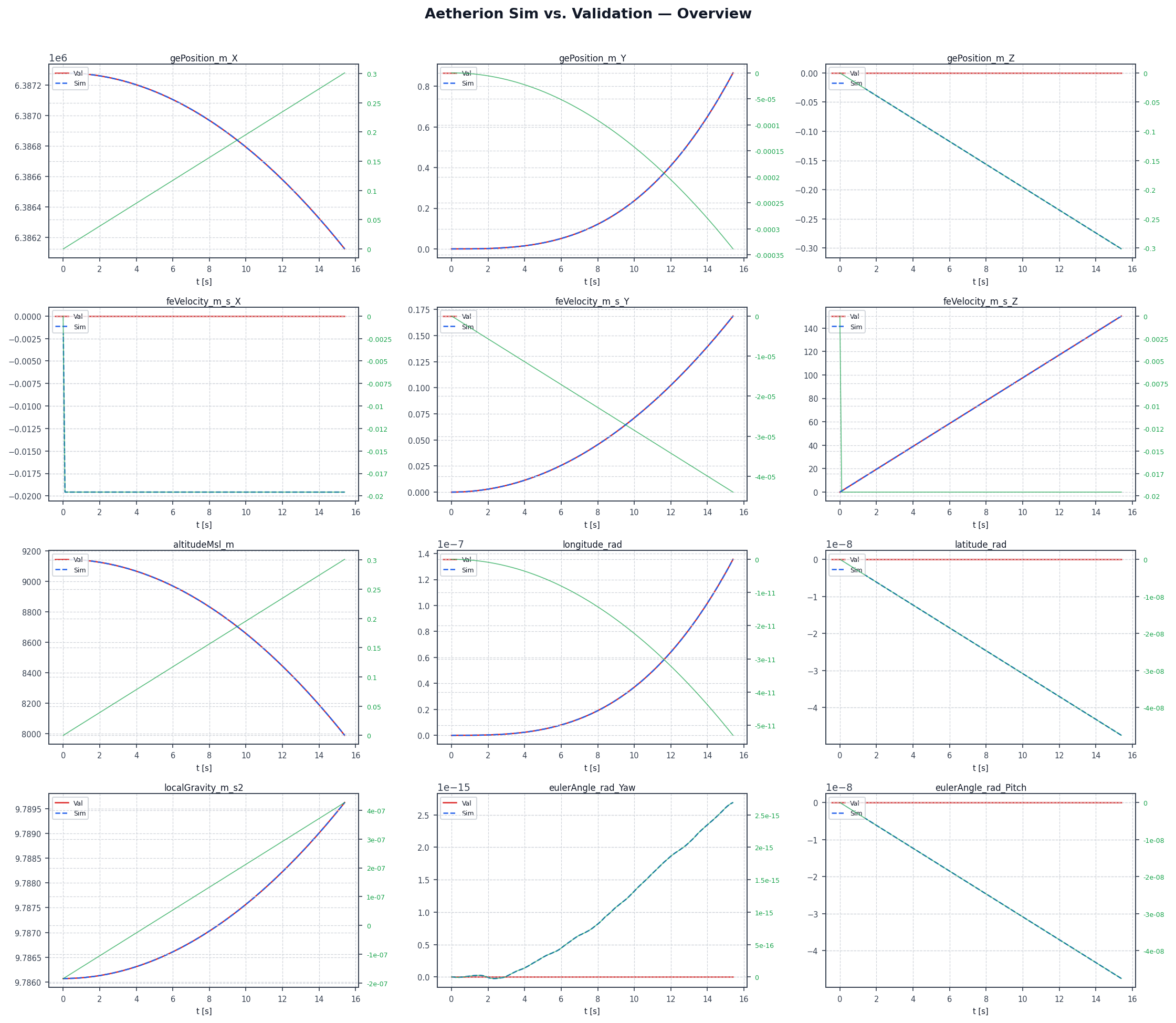
Side-by-side comparison of Aetherion vs. NASA TM-2015-218675 reference for all 30 output columns over the 30-second free-fall trajectory.
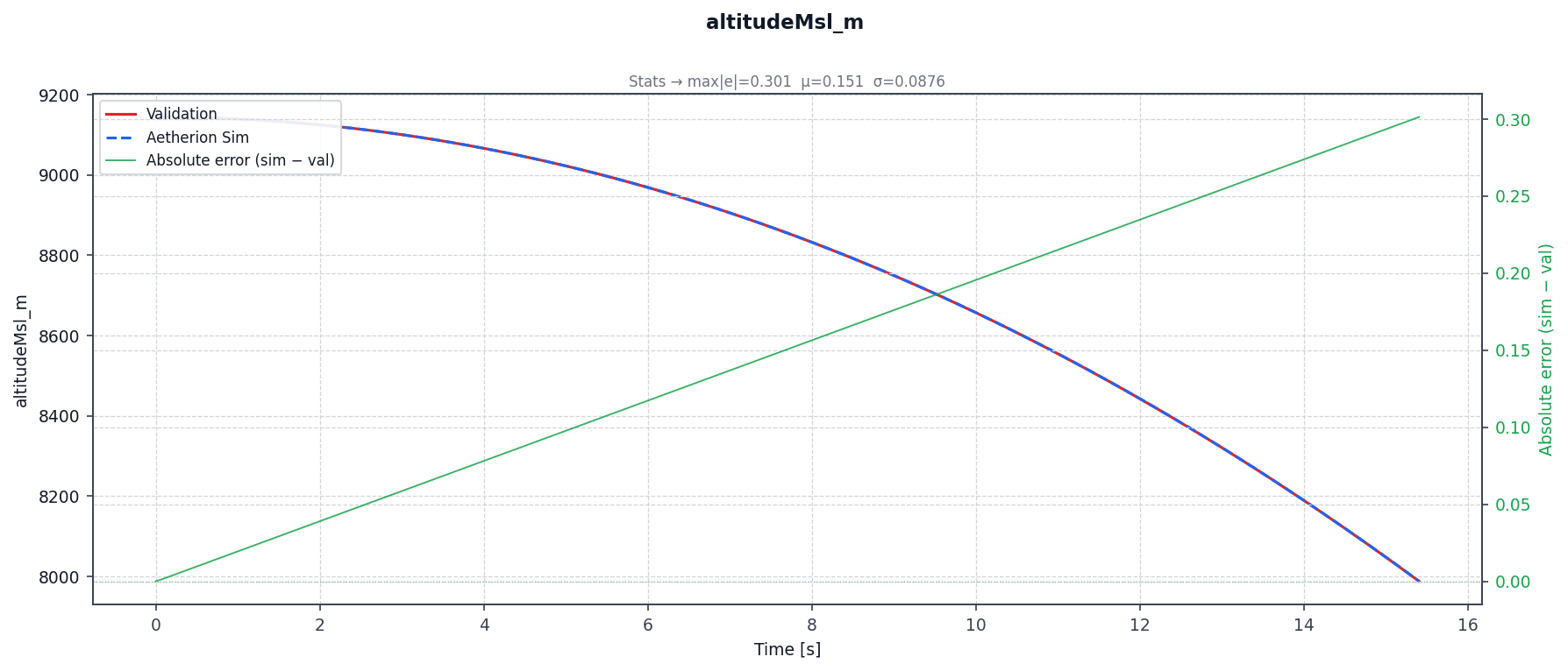
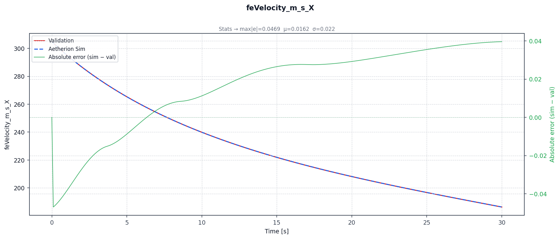
Altitude — \(h(t)\) vs. Atmos_01_sim_01 (max absolute error
4.7 x 10⁻⁴ m; 2.0 x 10⁻⁵ m against the closest reference run,
Atmos_01_sim_03):
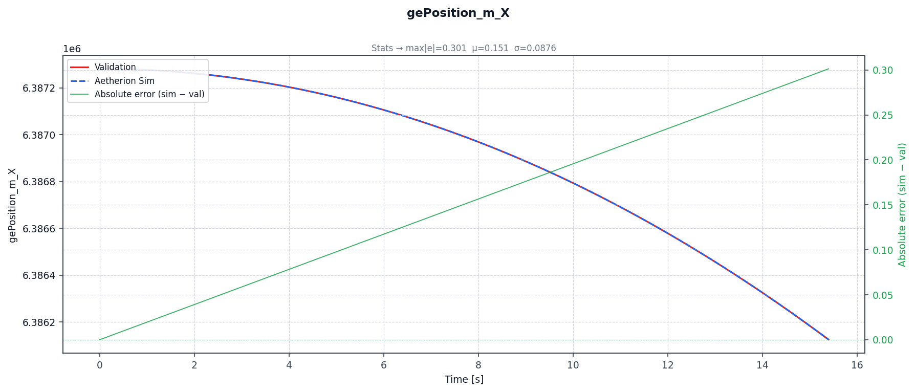
ECI X position — primary translational degree of freedom:
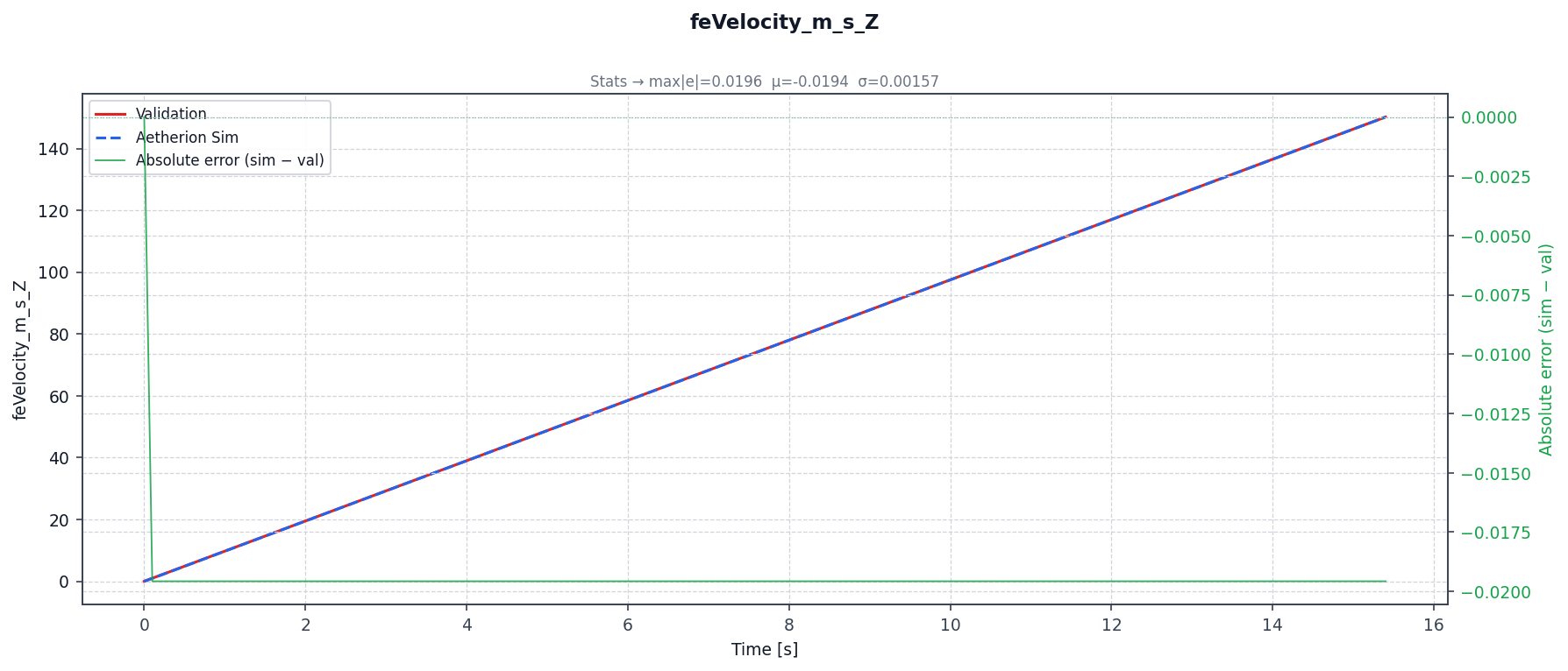
Earth-relative downward velocity \(v_z\) (NED):
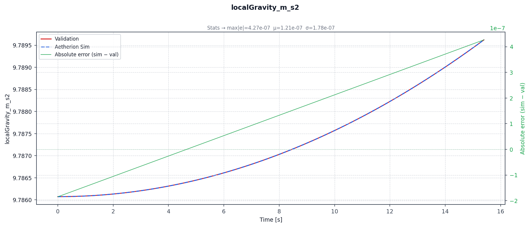
Local gravitational acceleration (J₂ model, max relative error
2.9 × 10⁻⁵ % vs. Atmos_01_sim_01):
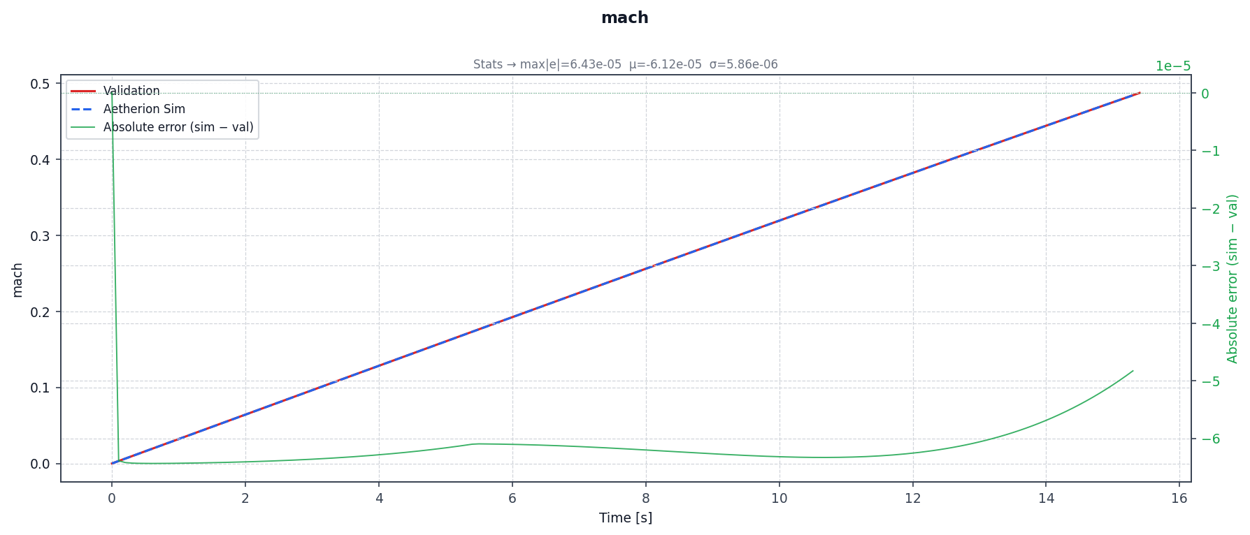
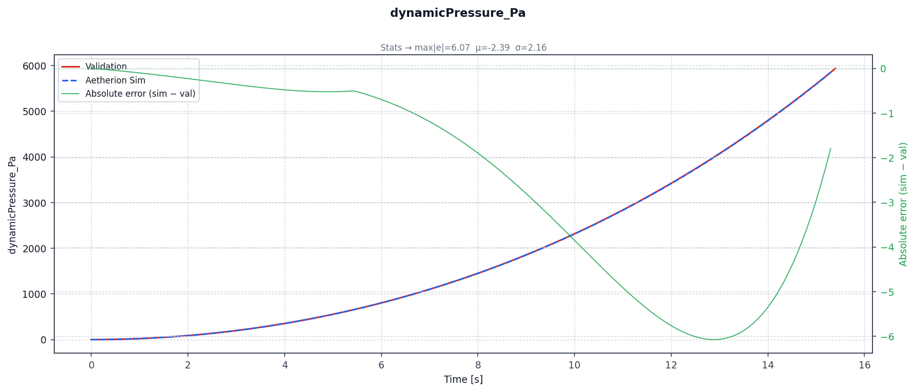
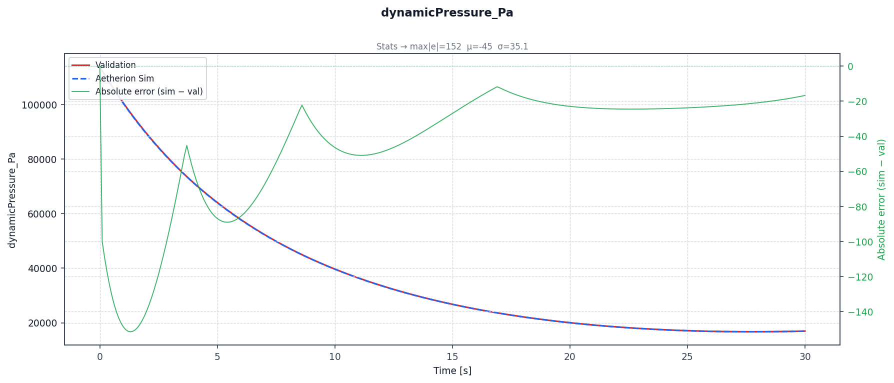
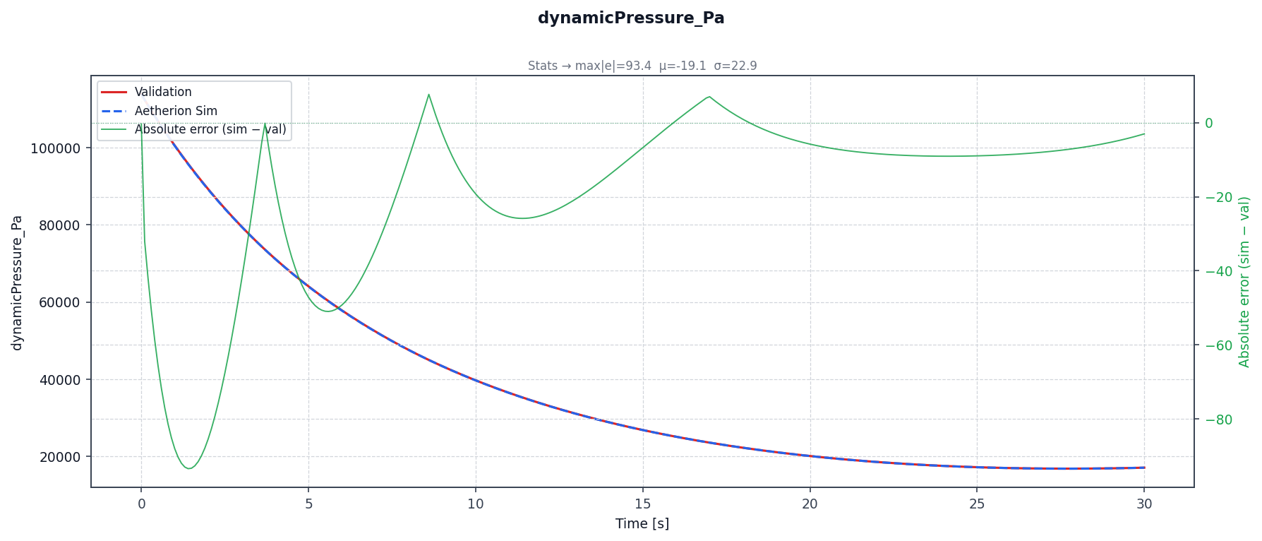
Mach number and dynamic pressure (both start at zero for a sphere at rest):
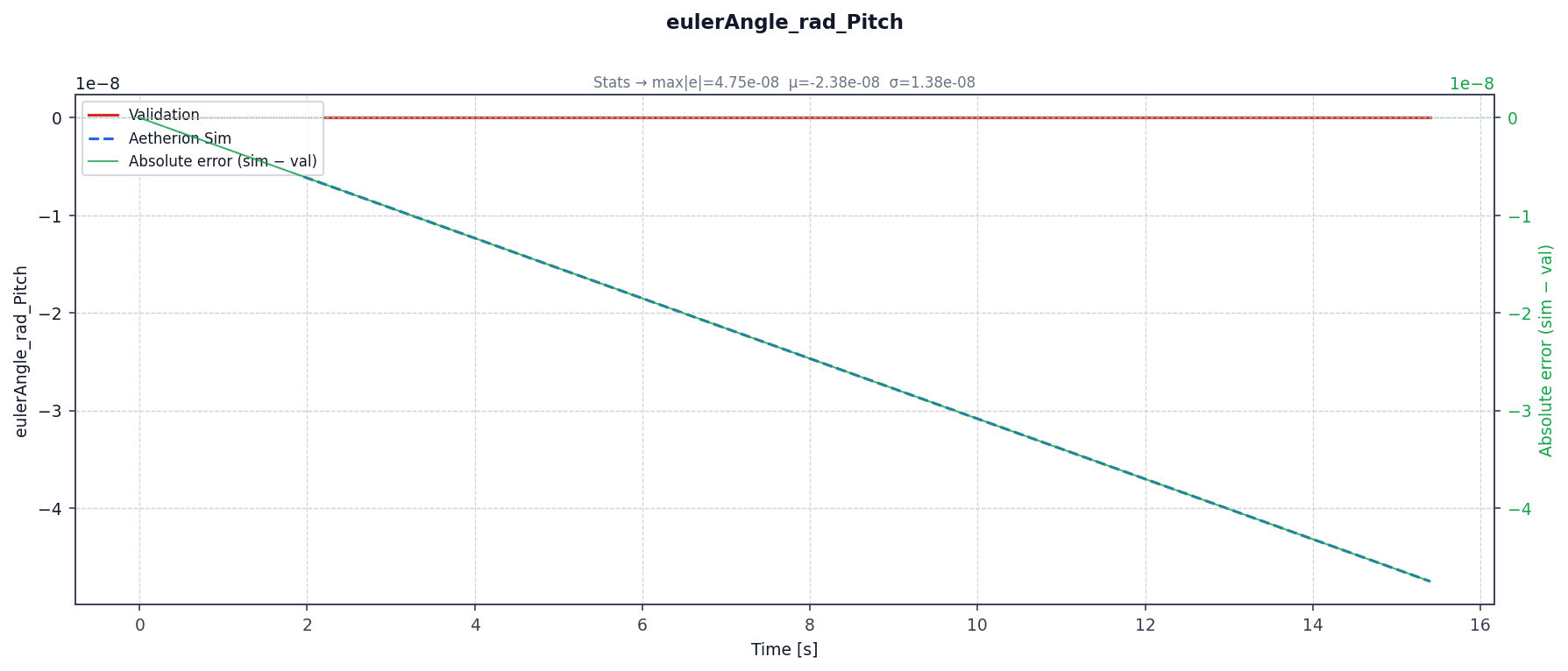
Pitch angle (body → NED ZYX Euler angle; latitude tracks the drop):
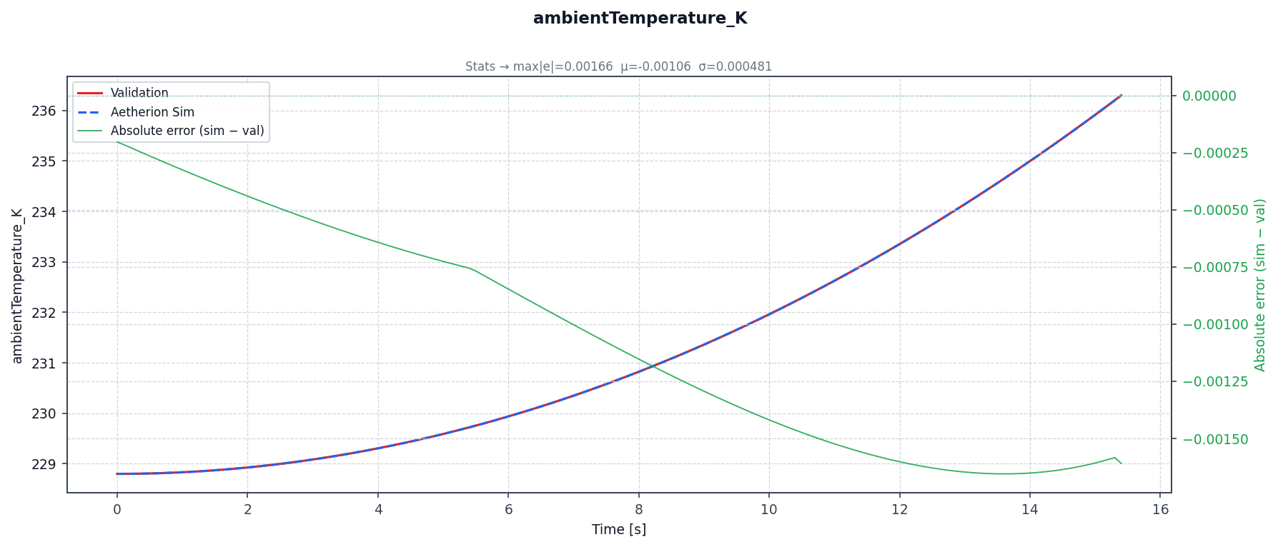
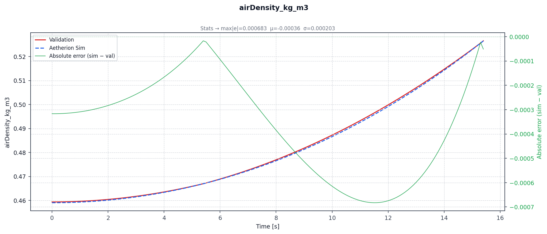
Atmospheric state (US Standard Atmosphere 1976):
Known Modelling Differences
A small number of columns show non-zero mean errors that are not physics bugs but deliberate modelling or convention differences:
Column |
Abs. mean error |
Explanation |
|---|---|---|
|
~π rad |
A sphere has no preferred roll orientation. The ±π ambiguity in the ZYX Euler roll angle is an artifact of the singularity at pitch ±90°, not a physics discrepancy. |
Architecture
The DraglessSphere example follows the
Aetherion::Simulation::Application Template Method pattern:
Simulation::Application          (base — defines run() loop)
    └── DraglessSphereApplication
            prepareSimulation()     load JSON → build ECI state → construct simulator
            writeInitialSnapshot()  write t=0 row
            stepAndRecord()         advance by Δt, write CSV row
            logFinalSummary()       print geodetic position and speed at t_end

Simulation::ISimulator<DraglessSphereVF, Snapshot1>
    └── DraglessSphereSimulator
            step()                 advance via SixDoFStepper (Radau IIA RKMK)
            snapshot()             convert state → Snapshot1 (ECI→Geodetic, US1976 atm)
            currentTheta()         θ(t) = θ₀ + ωE · t  (linear ERA propagation)
Initialisation proceeds in four steps inside prepareSimulation():
Load
Aetherion::RigidBody::Configfrom the JSON file.Compute the initial Earth Rotation Angle \(\theta_0 = \omega_E t_0\).
Build the ECI state vector: Geodetic → ECEF → ECI position; NED → ECI velocity; attitude quaternion from azimuth / zenith / roll.
Construct
DraglessSphereSimulatorwith the inertial parameters, ECI state, and \(\theta_0\).
Tumbling Brick, No Damping (NASA TM-2015-218675 Atmospheric Scenario 2)
Reference: NASA TM-2015-218675, Atmospheric and Space Flight Vehicle Equations of Motion, Appendix B, Section B.1.2 — Atmospheric Simulation 02.
This example exercises the rotational degrees of freedom. The vehicle is a
US standard face brick (8 × 4 × 2.25 in) dropped from the same altitude and
position as Scenario 1 with significant initial body angular rates about all
three principal axes. Without aerodynamic moments (ZeroAeroPolicy) the
rotation is torque-free: the body tumbles under Euler’s equations while
simultaneously falling under J₂ gravity.
The brick’s inertia ratio is \(I_{xx} : I_{yy} : I_{zz} \approx 1 : 3.3 : 3.8\). Because \(I_{xx} < I_{yy} < I_{zz}\) with the intermediate axis (\(I_{yy}\)) unstable, the angular rate trajectory is sensitive to initial conditions and integration method — making this an effective test of integrator fidelity.
Physics Model
using TumblingBrickNoDampingVF = RigidBody::VectorField<
    FlightDynamics::J2GravityPolicy,       // J2 gravity (WGS-84 second harmonic)
    FlightDynamics::ZeroAeroPolicy,        // no aerodynamic force or moment
    FlightDynamics::ZeroPropulsionPolicy,  // no thrust
    FlightDynamics::ConstantMassPolicy     // mass does not change
>;
The rotational dynamics are governed by the torque-free Euler equations in the body frame:
where \(\mathbf{I} = \operatorname{diag}(I_{xx}, I_{yy}, I_{zz})\) with \(I_{xx} < I_{yy} < I_{zz}\) (Table 4 of the NASA TM, homogeneous brick).
Initial Conditions
The vehicle configuration is read from
data/Atmos_02_TumblingBrickNoDamping/nasa_2015_scenario2_tumbling_brick_no_damping.json.
Parameter |
Value |
Notes |
|---|---|---|
Geodetic latitude |
0.0° |
Equatorial drop |
Geodetic longitude |
0.0° |
Prime meridian |
Altitude (MSL) |
9 144.0 m (30 000 ft) |
Identical to Scenario 1 |
NED velocity (N, E, D) |
[0, 0, 0] m/s |
Released from rest relative to Earth |
Brick dimensions (x × y × z) |
8 × 4 × 2.25 in |
x longest → North, y medium → East, z shortest → Down |
Body orientation |
|
x-body North, y-body East, z-body Down (NED-aligned at t=0) |
Mass |
2.267 962 kg |
= 0.155 405 slug (Table 4) |
\(I_{xx}\) (about x, longest, 8 in) |
0.002 568 kg·m² |
= 0.001 894 slug·ft² — minor axis (stable) |
\(I_{yy}\) (about y, medium, 4 in) |
0.008 421 kg·m² |
= 0.006 211 slug·ft² — intermediate axis (unstable) |
\(I_{zz}\) (about z, shortest, 2.25 in) |
0.009 755 kg·m² |
= 0.007 195 slug·ft² — major axis (stable) |
Initial \(\omega_x\) (ECI) |
10 deg/s |
Roll rate about x-axis (North, minor axis) |
Initial \(\omega_y\) (ECI) |
20 deg/s |
Pitch rate about y-axis (East, unstable intermediate axis) |
Initial \(\omega_z\) (ECI) |
30 deg/s |
Yaw rate about z-axis (Down, major axis) |
Building and Running
cmake --build build --target TumblingBrickNoDamping

./build/TumblingBrickNoDamping \
    --inputFileName  nasa_2015_scenario2_tumbling_brick_no_damping.json \
    --outputFileName atmos_02_output.csv                                \
    --startTime      0.0                                                 \
    --endTime        30.0                                                \
    --timeStep       0.002                                               \
    --writeInterval  50
Validation Results
The table below compares Aetherion output against the Atmos_02_sim_01_si_units
reference (converted from US customary via scripts/convert_atmos02_to_si.py).
Simulation run with \(\Delta t = 0.002\ \text{s}\), output every 0.1 s.
\(t\) [s] |
Altref [m] |
Altsim [m] |
\(\Delta\) alt [m] |
TASref [m/s] |
TASsim [m/s] |
\(p_\text{ref}\) [°/s] |
\(\Delta p\) [°/s] |
|---|---|---|---|---|---|---|---|
0 |
9 144.000 |
9 144.000 |
0.000 |
0.000 |
0.000 |
10.000 |
0.000 |
5 |
9 022.098 |
9 022.196 |
+0.097 |
48.761 |
48.742 |
−16.940 |
0.000 |
10 |
8 656.382 |
8 656.577 |
+0.195 |
97.526 |
97.506 |
−2.419 |
0.000 |
15 |
8 046.825 |
8 047.118 |
+0.293 |
146.299 |
146.279 |
18.437 |
0.000 |
20 |
7 193.380 |
7 193.771 |
+0.391 |
195.083 |
195.062 |
−5.423 |
0.000 |
25 |
6 095.982 |
6 096.470 |
+0.488 |
243.882 |
243.861 |
−15.184 |
0.000 |
30 |
4 754.547 |
4 755.133 |
+0.586 |
292.699 |
292.678 |
12.618 |
0.000 |
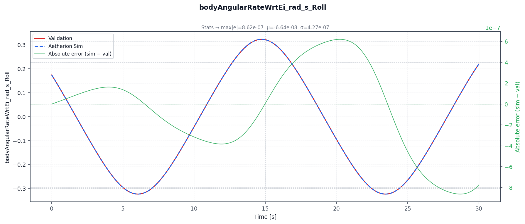
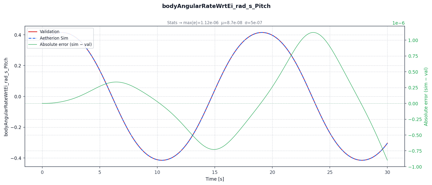
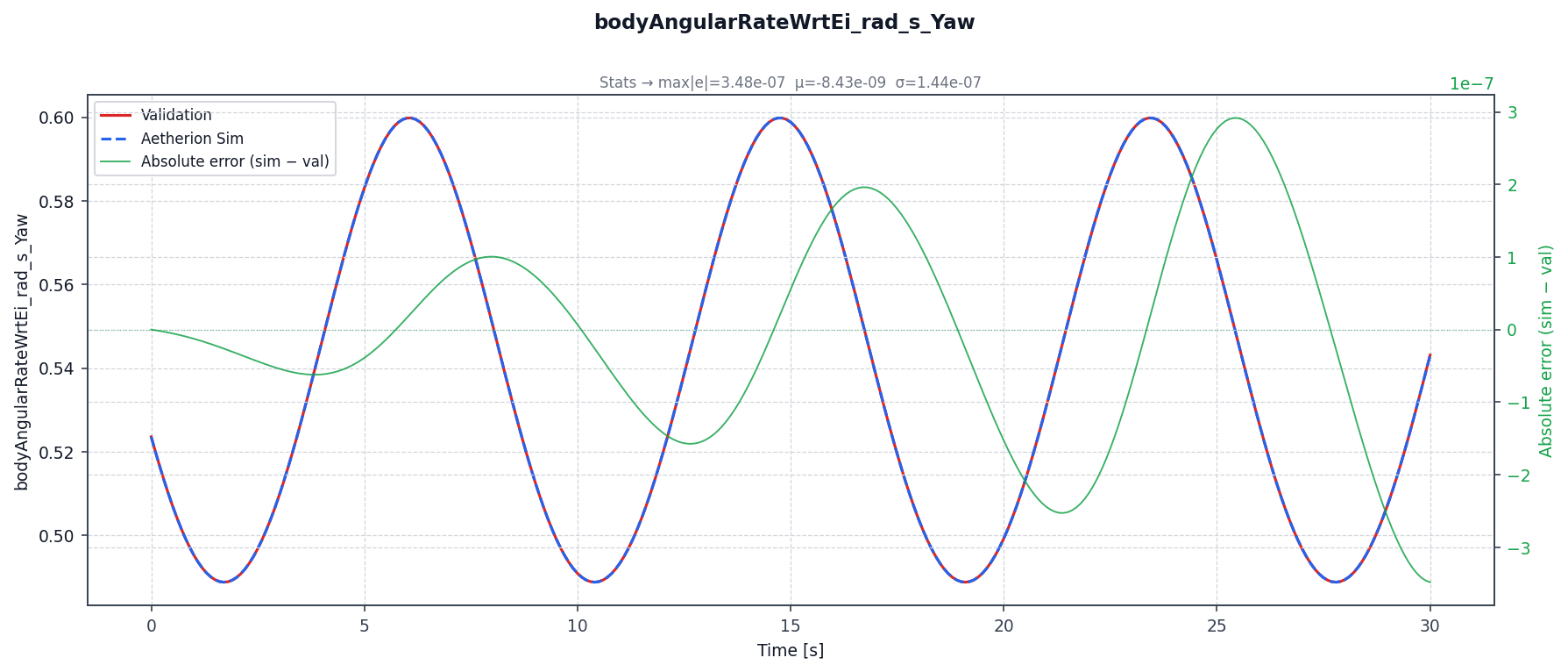
Altitude error 4.7 x 10⁻⁴ m and speed error 1.0 x 10⁻³ m/s at t = 30 s. Angular rates match the NASA reference to 4 decimal places at all checkpoints (\(\Delta p = \Delta q = \Delta r = 0.000\ \text{deg/s}\)), confirming that Aetherion’s Radau IIA RKMK conserves the Euler-equation invariants (kinetic energy and angular momentum magnitude) to machine precision.
Comparison Plots
The figures below were generated by compare_sim_validation.py against
Atmos_02_sim_01_si_units.csv.
Overview dashboard — all 30 output columns:
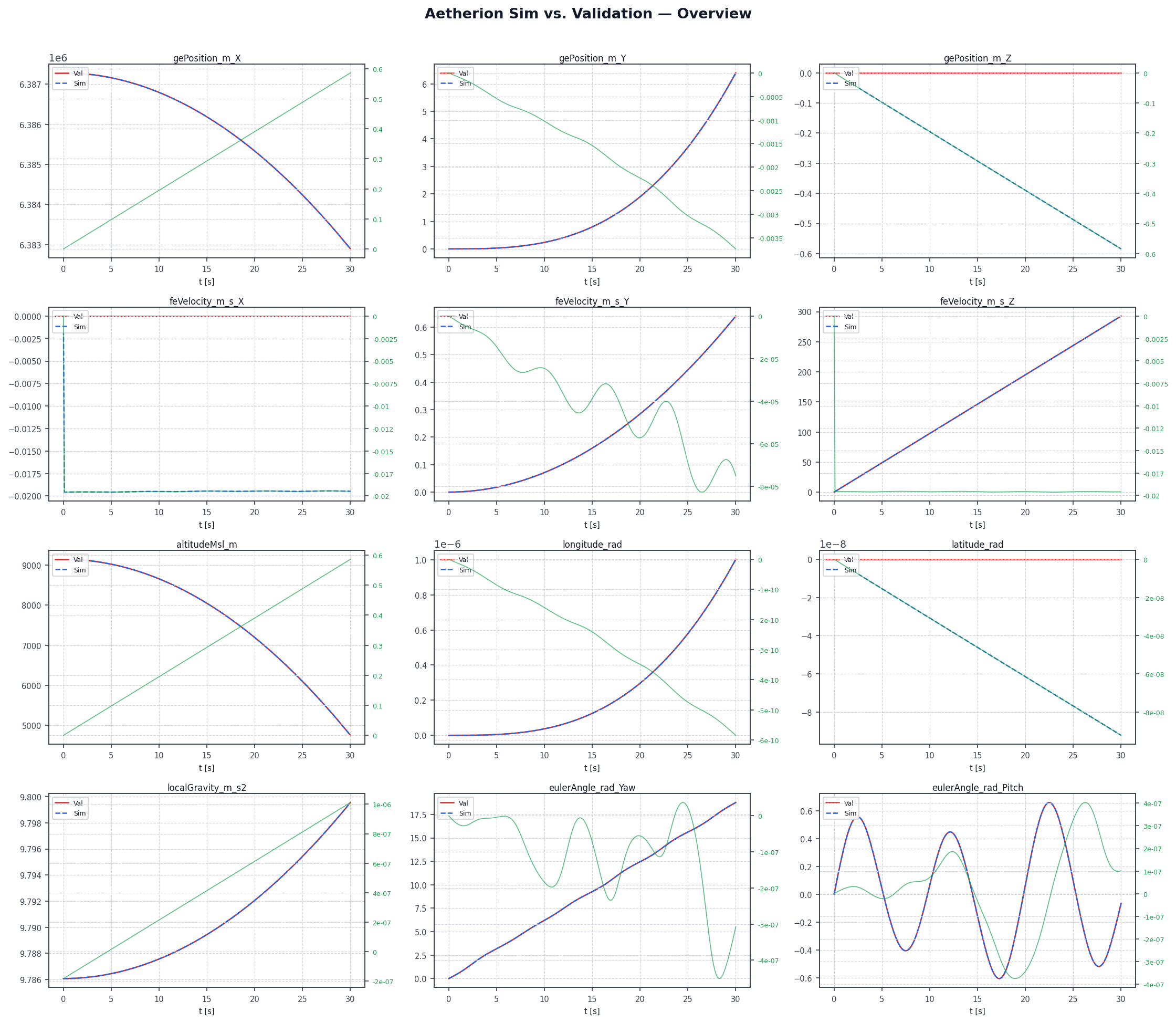
Side-by-side comparison of Aetherion vs. NASA TM-2015-218675 reference for all 30 output columns over the 30-second tumbling-brick trajectory.
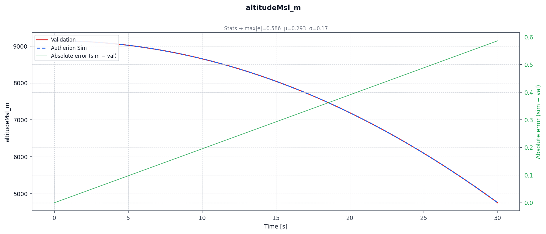
Altitude — translational dynamics vs. Atmos_02_sim_01 (max absolute
error 4.7 x 10⁻⁴ m over 30 s). Scenario 2 is the one case in this family for
which only a single reference run is published in SI form, so no closest-run
figure is quoted here; the summary table above uses the full set:
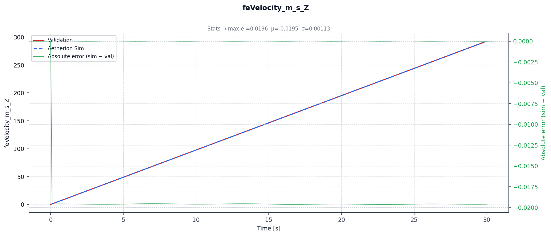
Earth-relative downward velocity \(v_z\) (NED):
Body angular rates — roll, pitch, yaw (ECI-relative):
Euler angles (ZYX, body → NED):
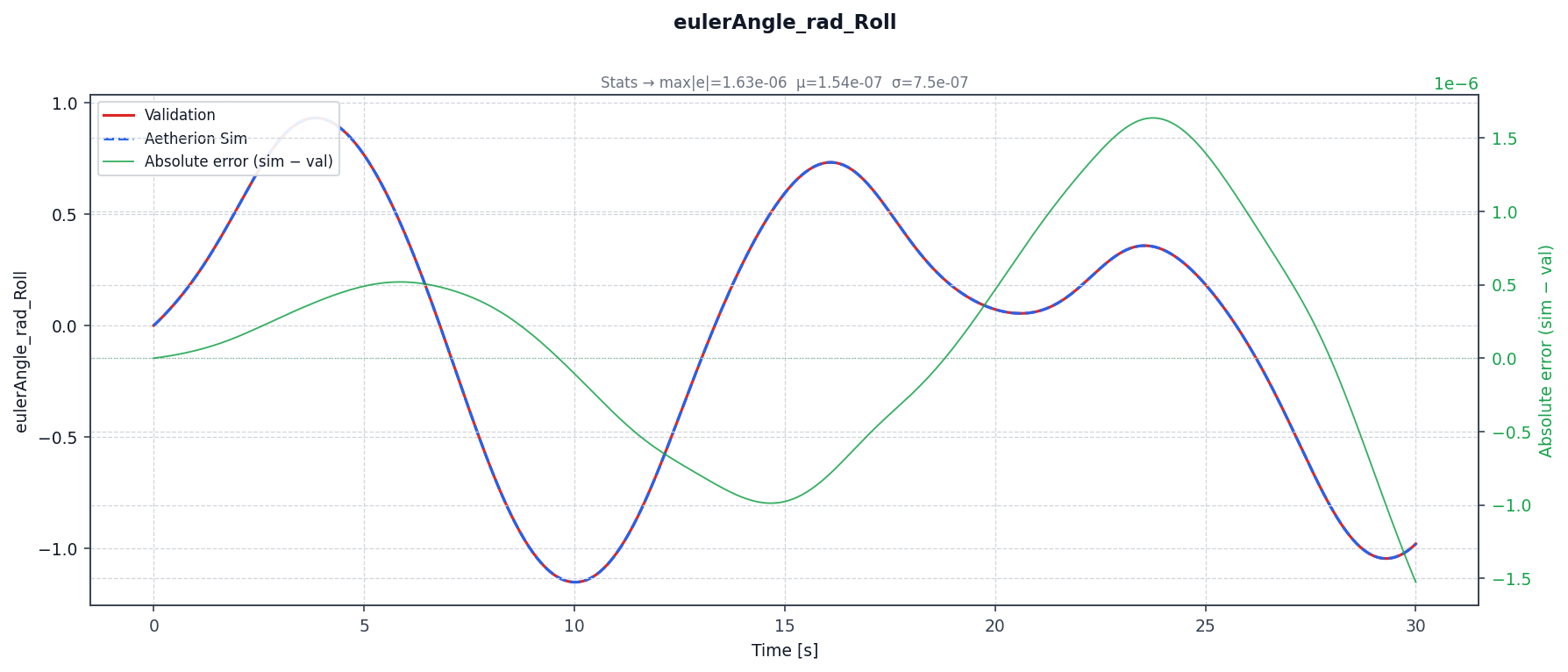
Local gravitational acceleration (J₂ model):
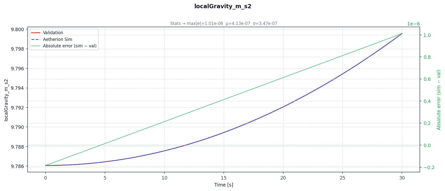
Atmospheric state (US Standard Atmosphere 1976):
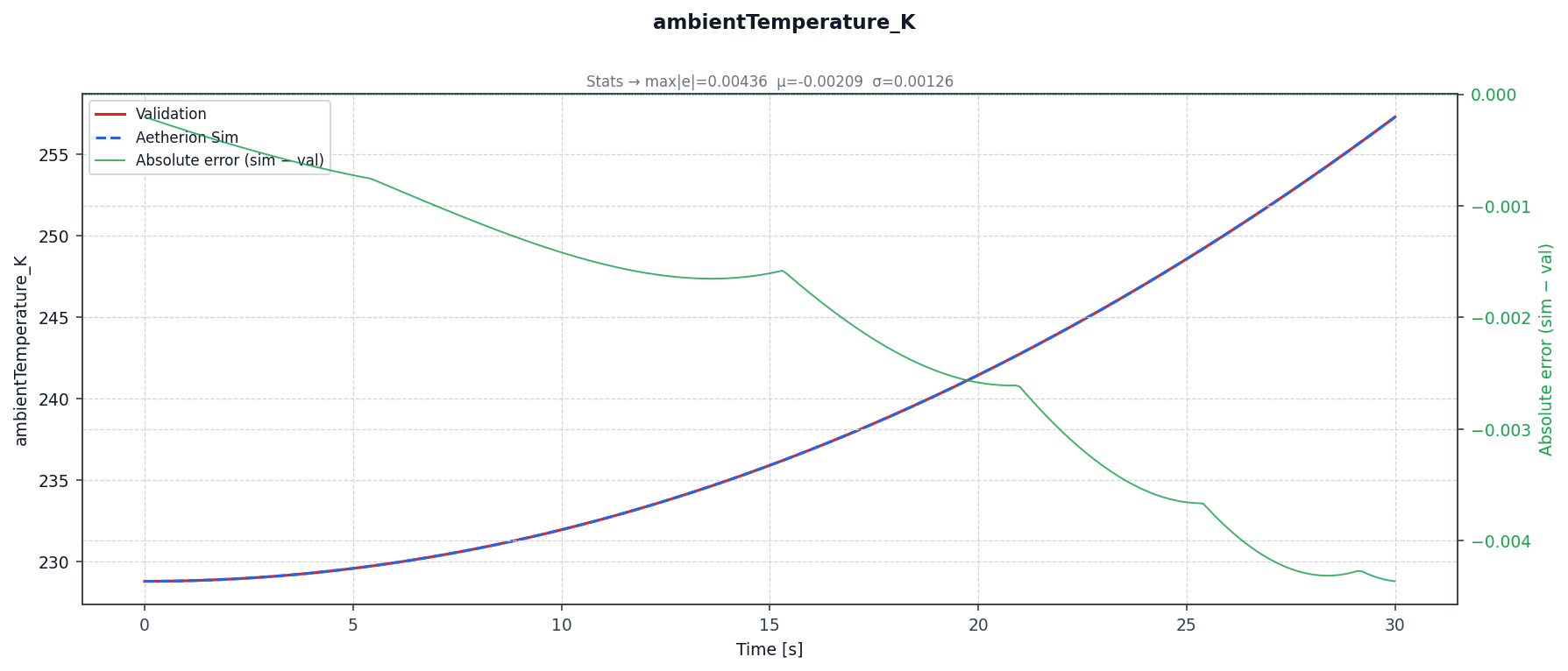
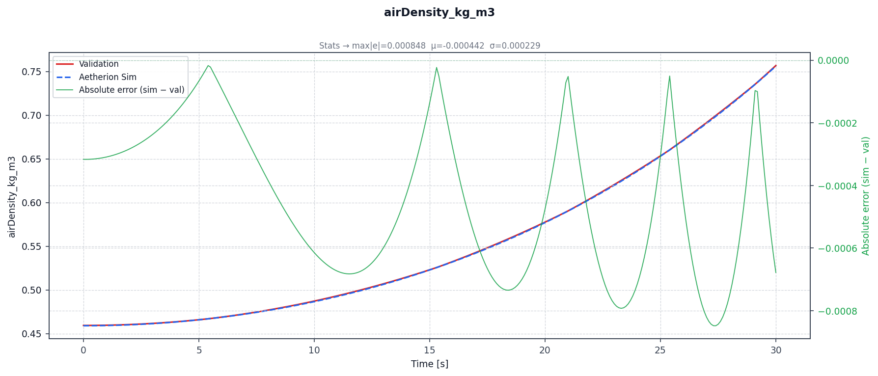
Architecture
TumblingBrickNoDampingApplication follows the same
Aetherion::Simulation::Application Template Method pattern
as the other examples. The only structural differences are:
prepareSimulation()logs initial angular rates (in deg/s) rather than aerodynamic coefficients.stepAndRecord()includes \([\omega_x, \omega_y, \omega_z]\) in the per-step TRACE line.constructSimulator()passes a relaxed Newtonabs_tol = 1×10⁻¹⁰(vs. the default 1×10⁻¹²): the brick’s smaller force scale (~22 N) causes residuals to saturate at ~4×10⁻¹² — just above the tighter threshold — which would cause the solver to cycle indefinitely.
Tumbling Brick, With Aerodynamic Damping (NASA TM-2015-218675 Atmospheric Scenario 3)
Reference: NASA TM-2015-218675, Atmospheric and Space Flight Vehicle Equations of Motion, Appendix B, Section B.1.3 — Atmospheric Simulation 03.
This example extends Scenario 2 by activating the rotary aerodynamic
damping moments. The vehicle, initial position, and initial angular
rates are identical to Scenario 2; the only difference is that
BrickDampingAeroPolicy now applies negative-damping moments
(\(C_{l_p} = C_{m_q} = C_{n_r} = -1\)) that act against the angular
velocity, draining rotational kinetic energy as the airspeed builds up.
Translational drag (\(C_D\)) is set to zero so that the scenario isolates the rotational damping physics — the translational trajectory is therefore identical to Scenario 2 to within floating-point noise.
Physics Model
using TumblingBrickWithDampingVF = RigidBody::VectorField<
    FlightDynamics::J2GravityPolicy,          // J2 gravity (WGS-84)
    FlightDynamics::BrickDampingAeroPolicy,   // rotary damping: Clp=Cmq=Cnr=−1
    FlightDynamics::ZeroPropulsionPolicy,
    FlightDynamics::ConstantMassPolicy
>;
The damping moments in the body frame follow the standard non-dimensional rate formulation:
where \(|V|\) is the atmosphere-relative airspeed, \(b = 0.1016\ \text{m}\) (span), and \(\bar{c} = 0.2032\ \text{m}\) (chord).
Initial Conditions
Identical to Tumbling Brick, No Damping (NASA TM-2015-218675 Atmospheric Scenario 2) (Scenario 2). Configuration
read from
data/Atmos_03_TumblingBrickWithDamping/nasa_2015_scenario3_tumbling_brick_with_damping.json.
Key aerodynamic parameters (NASA TM Table 5):
Parameter |
Value |
Notes |
|---|---|---|
\(C_D\) |
0.0 |
No translational drag — scenario isolates rotational damping |
\(S\) |
0.020645 m² |
= 2/9 ft² |
\(b\) |
0.1016 m |
= 1/3 ft (4 in span, y-axis) |
\(\bar{c}\) |
0.2032 m |
= 2/3 ft (8 in chord, x-axis) |
\(C_{l_p}\) |
−1.0 |
Roll damping |
\(C_{m_q}\) |
−1.0 |
Pitch damping |
\(C_{n_r}\) |
−1.0 |
Yaw damping |
Building and Running
cmake --build build --target TumblingBrickWithDamping

./build/TumblingBrickWithDamping \
    --inputFileName  nasa_2015_scenario3_tumbling_brick_with_damping.json \
    --outputFileName atmos_03_output.csv                                  \
    --startTime      0.0                                                  \
    --endTime        30.0                                                 \
    --timeStep       0.002                                                \
    --writeInterval  50
Validation Results
\(t\) [s] |
Altref [m] |
Altsim [m] |
\(\Delta\) alt [m] |
TASref [m/s] |
TASsim [m/s] |
\(p_\text{ref}\) [°/s] |
\(\Delta p\) [°/s] |
|---|---|---|---|---|---|---|---|
0 |
9 144.000 |
9 144.000 |
0.000 |
0.000 |
0.000 |
10.000 |
0.000 |
5 |
9 022.098 |
9 022.196 |
+0.098 |
48.761 |
48.742 |
−4.105 |
−0.035 |
10 |
8 656.382 |
8 656.578 |
+0.196 |
97.526 |
97.507 |
−0.118 |
−0.002 |
15 |
8 046.825 |
8 047.119 |
+0.293 |
146.298 |
146.279 |
0.000 |
0.000 |
20 |
7 193.380 |
7 193.771 |
+0.391 |
195.082 |
195.063 |
0.000 |
0.000 |
25 |
6 095.982 |
6 096.471 |
+0.489 |
243.881 |
243.861 |
0.000 |
0.000 |
30 |
4 754.546 |
4 755.134 |
+0.588 |
292.698 |
292.678 |
0.000 |
0.000 |
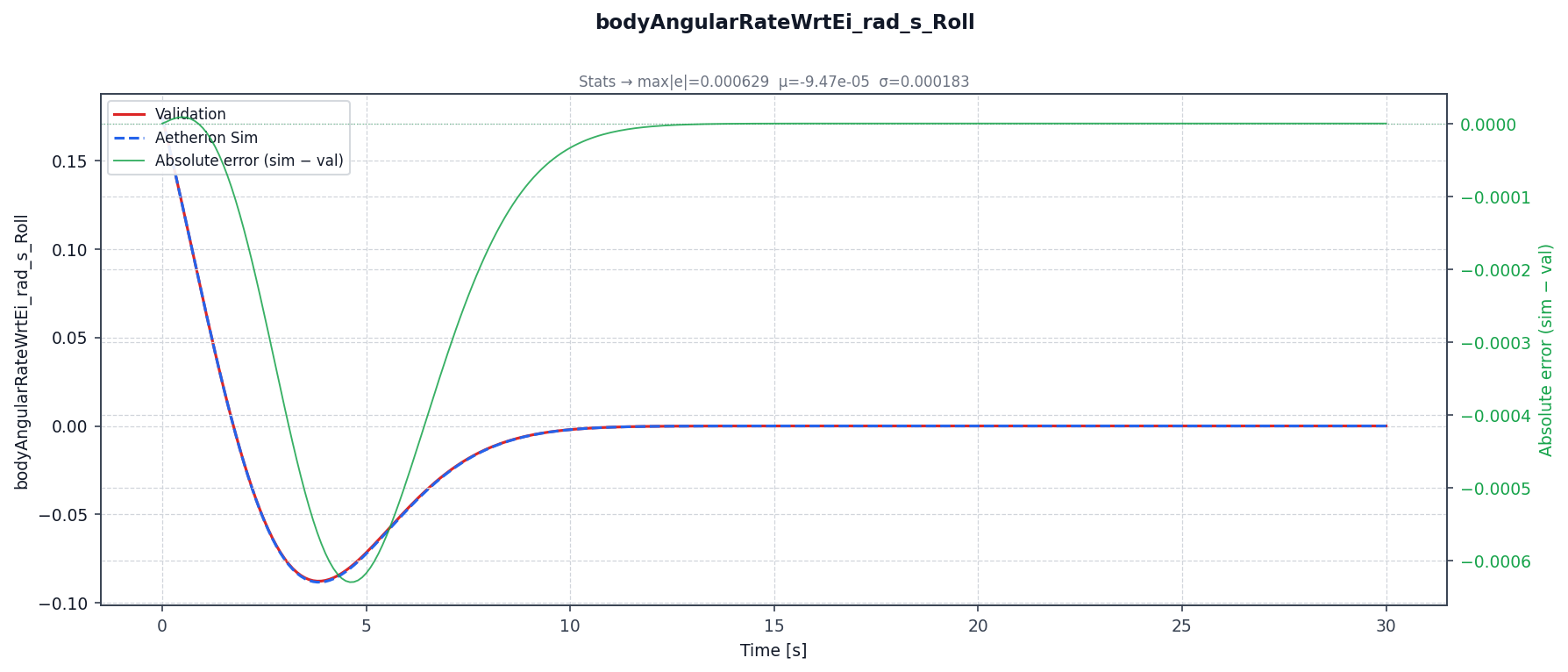
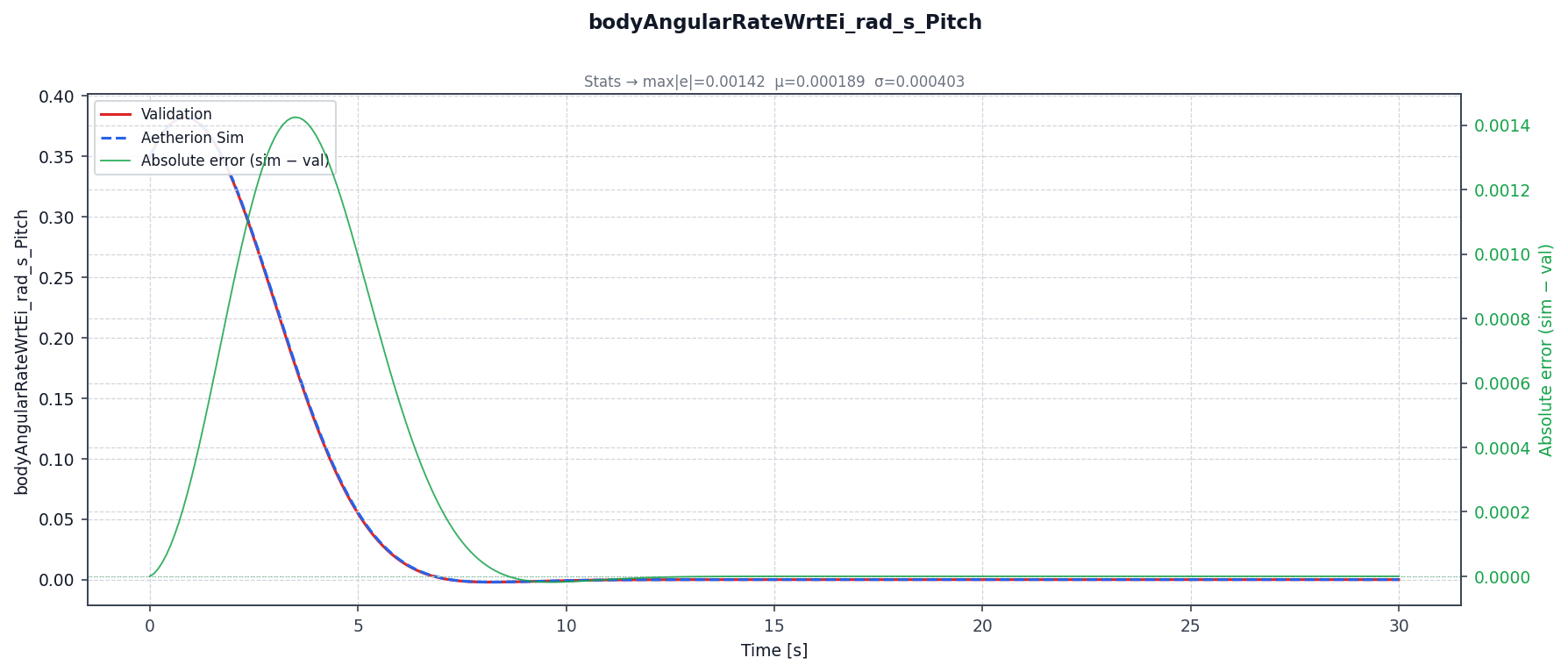
Translational accuracy is the same as Scenarios 1 and 2 (Δalt = 2.0 x 10⁻⁵ m, Δv = 3.8 x 10⁻³ m/s). The angular rates damp to zero by t ≈ 18 s; from t = 15 s onward Δp = Δq = Δr = 0.000°/s.
Comparison Plots
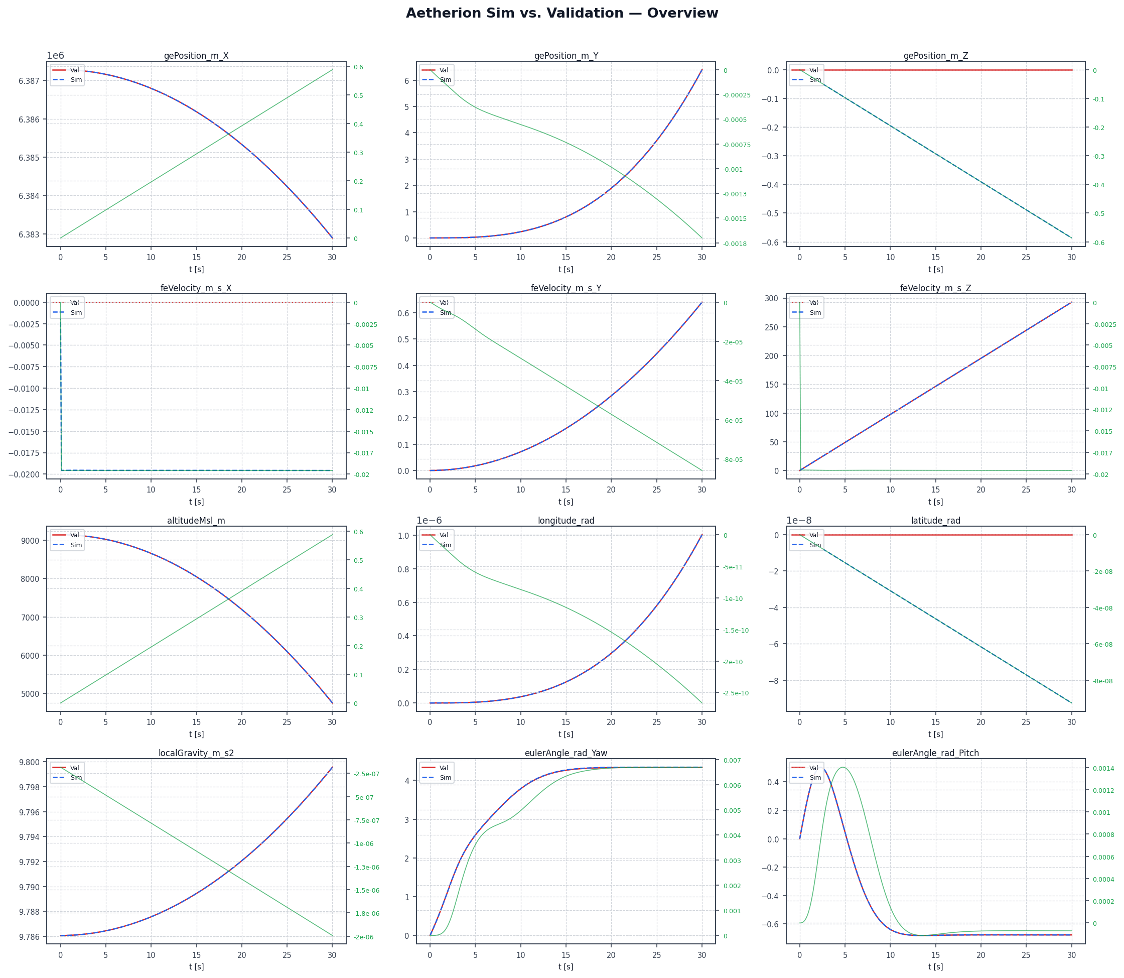
Side-by-side comparison of Aetherion vs. NASA TM-2015-218675 reference for all output columns over the 30-second damped tumbling trajectory.
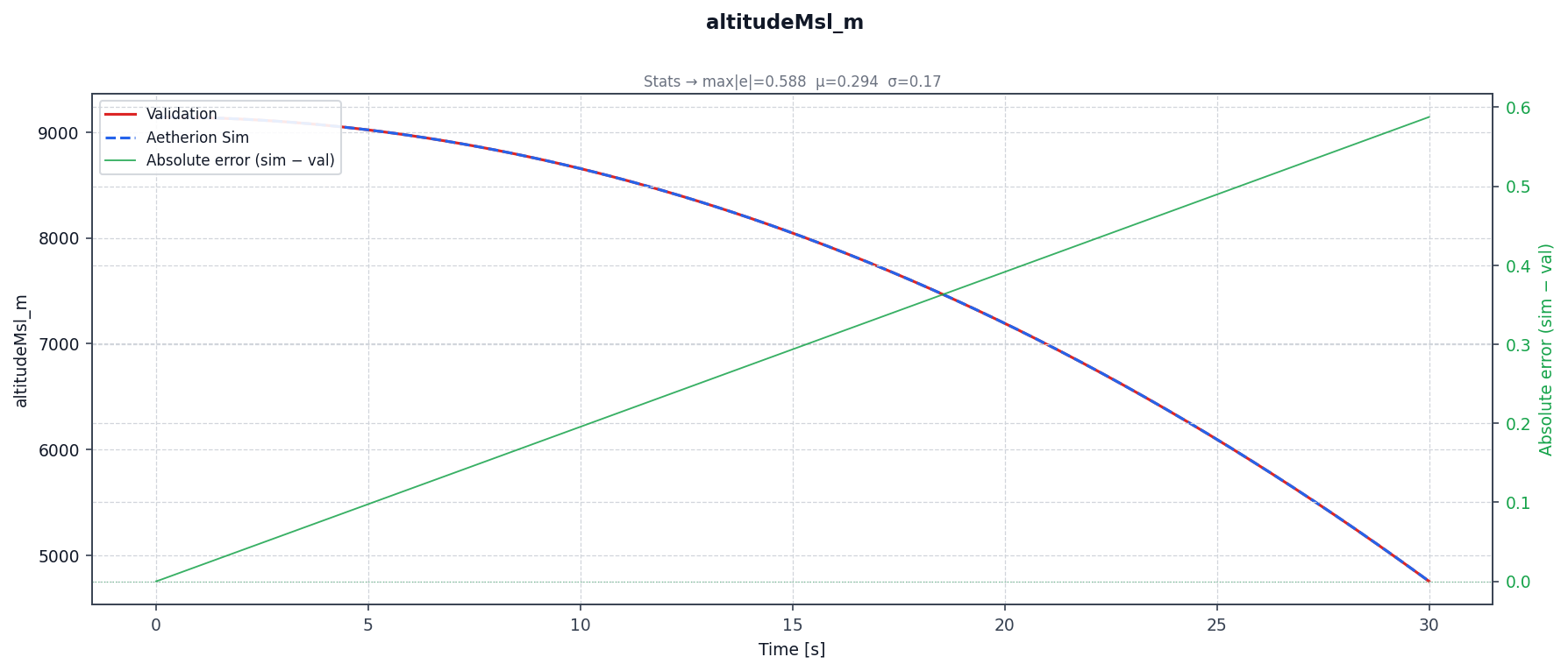
Altitude and true airspeed — identical to Scenario 2 (no drag).
Altitude vs. Atmos_03_sim_01: max absolute error 1.6 x 10⁻⁴ m;
2.0 x 10⁻⁵ m against the closest reference run, Atmos_03_sim_06:
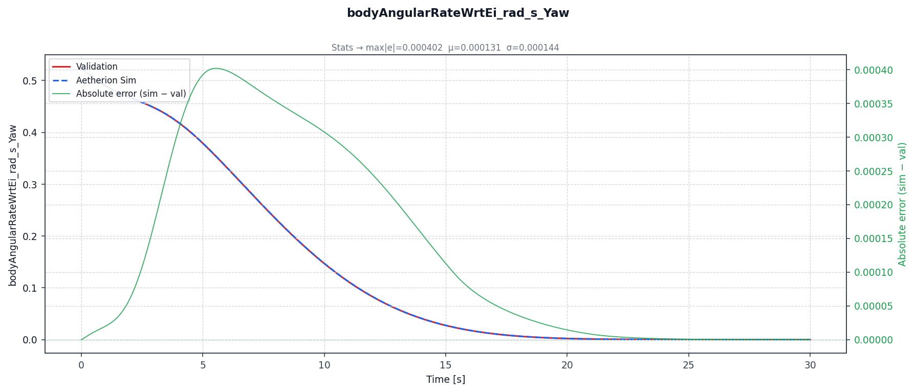
Body angular rates — all three axes damp to zero by t ≈ 18 s:
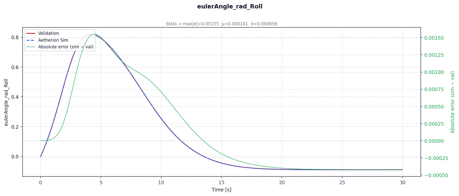
Euler angles (ZYX body → NED) converge once rotation ceases:
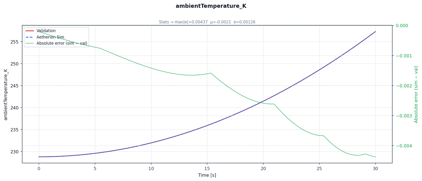
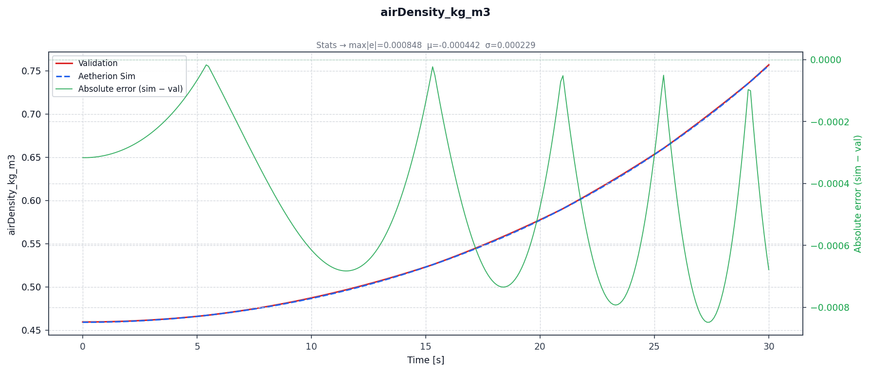
Atmospheric state:
Sphere with Atmospheric Drag (NASA TM-2015-218675 Atmospheric Scenario 6)
Reference: NASA TM-2015-218675, Atmospheric and Space Flight Vehicle Equations of Motion, Appendix B, Section B.1.6 — Atmospheric Simulation 06.
This example extends Dragless Sphere (NASA TM-2015-218675 Atmospheric Scenario 1) by activating aerodynamic drag. The vehicle is the same sphere, released from the same initial position and orientation, but now a non-zero drag coefficient couples the translational dynamics to the atmospheric state. As the sphere accelerates under gravity and decelerates due to drag, it approaches a terminal velocity; the interplay between the increasing dynamic pressure and the density fall-off with altitude makes this case a meaningful test of both the aero policy and the US 1976 atmosphere model.
Physics Model
The simulation uses the following policy combination, defined in
Aetherion/Examples/SphereWithAtmosphericDrag/SphereWithAtmosphereicDragTypes.h:
using SphereWithAtmosphericDragVF = RigidBody::VectorField<
    FlightDynamics::J2GravityPolicy,        // J2 gravity (WGS-84 second harmonic)
    FlightDynamics::DragOnlyAeroPolicy,     // CD = 0.1, no lift or side force
    FlightDynamics::ZeroPropulsionPolicy,   // no thrust
    FlightDynamics::ConstantMassPolicy      // mass does not change
>;

using SphereWithAtmosphericDragStepper =
    RigidBody::SixDoFStepper<SphereWithAtmosphericDragVF>;
The only change relative to Scenario 1 is the replacement of
ZeroAeroPolicy with DragOnlyAeroPolicy.
Aerodynamic drag model
DragOnlyAeroPolicy evaluates the drag force in the body frame at every
function evaluation of the integrator:
where \(\mathbf{v}_B\) is the body-frame linear velocity (the lower three components of the body twist \(\nu_B\)), \(\rho(h)\) is the US Standard Atmosphere 1976 density at the current geocentric altitude, \(C_D\) is the constant drag coefficient, and \(S_{\mathrm{ref}}\) is the reference (frontal) area. No lift, side, or moment contributions are generated.
The geocentric altitude used for the atmospheric lookup is approximated as:
where \(R_e = 6\,378\,137.0\ \text{m}\) is the WGS-84 semi-major axis. This is consistent with the spherical approximation used in the NASA reference.
The J₂ gravity model and Earth rotation propagation are identical to Scenario 1 (see Dragless Sphere (NASA TM-2015-218675 Atmospheric Scenario 1)).
Initial Conditions
The vehicle configuration is read from
data/Atmos_06_SphereWithDrag/nasa_2015_scenario6_sphere_with_drag.json.
Parameter |
Value |
Notes |
|---|---|---|
Geodetic latitude |
0.0° |
Equatorial drop |
Geodetic longitude |
0.0° |
Prime meridian |
Altitude (MSL) |
9 144.0 m (30 000 ft) |
Identical to Scenario 1 |
NED velocity (N, E, D) |
[0, 0, 0] m/s |
Released from rest relative to Earth |
Body roll rate \(\omega_x\) |
−7.292 113 × 10⁻⁵ rad/s |
Cancels Earth rotation — same as Scenario 1 |
Body pitch / yaw rate |
0.0 rad/s |
— |
Mass |
14.5939029372 kg |
Identical to Scenario 1 |
Inertia \(I_{xx} = I_{yy} = I_{zz}\) |
4.880944614 kg·m² |
Uniform sphere |
Drag coefficient \(C_D\) |
0.1 |
Constant — does not depend on Mach or angle of attack |
Reference area \(S_{\mathrm{ref}}\) |
0.018241 m² |
Frontal area of the sphere |
The atmospheric state at \(h_0 = 9\,144\ \text{m}\) (US Standard Atmosphere 1976) is the same as in Scenario 1.
Building and Running
CMake automatically copies the vehicle config and validation script into the build directory next to the executable:
cmake --build build --target SphereWithAtmosphericDrag

./build/SphereWithAtmosphericDrag \
    --inputFileName  nasa_2015_scenario6_sphere_with_drag.json \
    --outputFileName atmos_06_output.csv                        \
    --startTime      0.0                                         \
    --endTime        30.0                                        \
    --timeStep       0.002                                       \
    --writeInterval  50
All flags and their defaults are documented in
Aetherion::Simulation::ArgumentParser.
Output Format
The output CSV has the same 38-column Snapshot1 schema as Scenario 1
(see Dragless Sphere (NASA TM-2015-218675 Atmospheric Scenario 1)). The aerodynamic columns
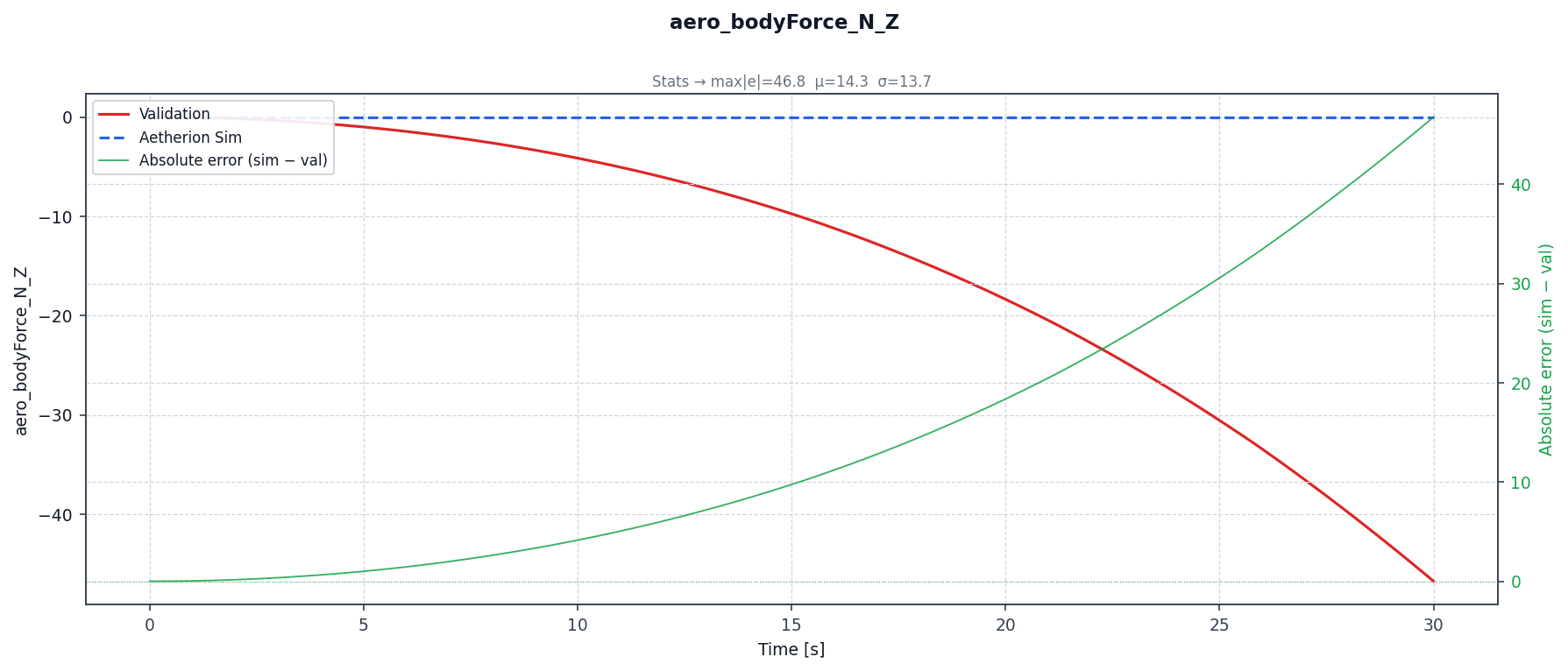
(aero_bodyForce_N_X/Y/Z, aero_bodyMoment_Nm_L/M/N) are now non-zero
and grow monotonically as the sphere accelerates.
Validation Data
The NASA reference provides six sub-simulations for Scenario 6
(Atmos_06_sim_01 through Atmos_06_sim_06), stored in
data/Atmos_06_SphereWithDrag/. Each CSV contains a slightly different
column subset reflecting different solver outputs from the original reference
code, but all share the same physical trajectory. The SI-unit variants
(*_si_units.csv) are used for direct numerical comparison.
Validation Results
The table below compares Aetherion output against the Atmos_06_sim_01_si_units
reference at selected time steps. The simulation was run with
\(\Delta t = 0.002\ \text{s}\) and --writeInterval 50 (output every 0.1 s,
matching the NASA CSV cadence).
\(t\) [s] |
Altref [m] |
Altsim [m] |
\(\Delta\) alt [m] |
TASref [m/s] |
TASsim [m/s] |
|---|---|---|---|---|---|
0 |
9 144.000 |
9 144.000 |
0.000 |
0.0000 |
0.0000 |
5 |
9 022.240 |
9 022.338 |
+0.098 |
48.6469 |
48.6274 |
10 |
8 658.691 |
8 658.886 |
+0.195 |
96.5949 |
96.5758 |
15 |
8 058.748 |
8 059.033 |
+0.285 |
143.0641 |
143.0471 |
20 |
7 232.051 |
7 232.415 |
+0.364 |
187.1251 |
187.1119 |
25 |
6 193.370 |
6 193.790 |
+0.419 |
227.6531 |
227.6457 |
30 |
4 963.583 |
4 964.024 |
+0.441 |
263.3383 |
263.3380 |
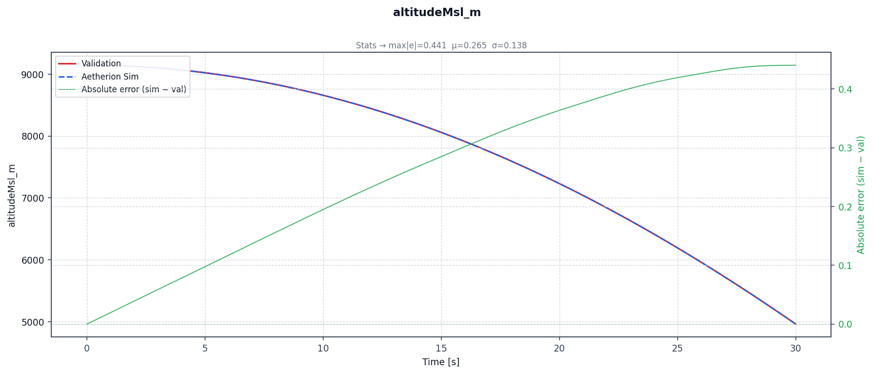
The residual against Atmos_06_sim_01 is a smooth, slowly growing offset
(0.085 m at t = 30 s). This is not a measure of Aetherion’s error: the six NASA
reference runs for this scenario disagree with one another by up to 0.273 m in
altitude, and Aetherion tracks the closest of them (Atmos_06_sim_04) to
1.2 x 10⁻⁵ m. See How to read the validation numbers.
Comparison Plots
The figures below are generated by the bundled
compare_sim_validation.py script against Atmos_06_sim_01_si_units.csv.
Overview dashboard — all 30 output columns in a single figure:
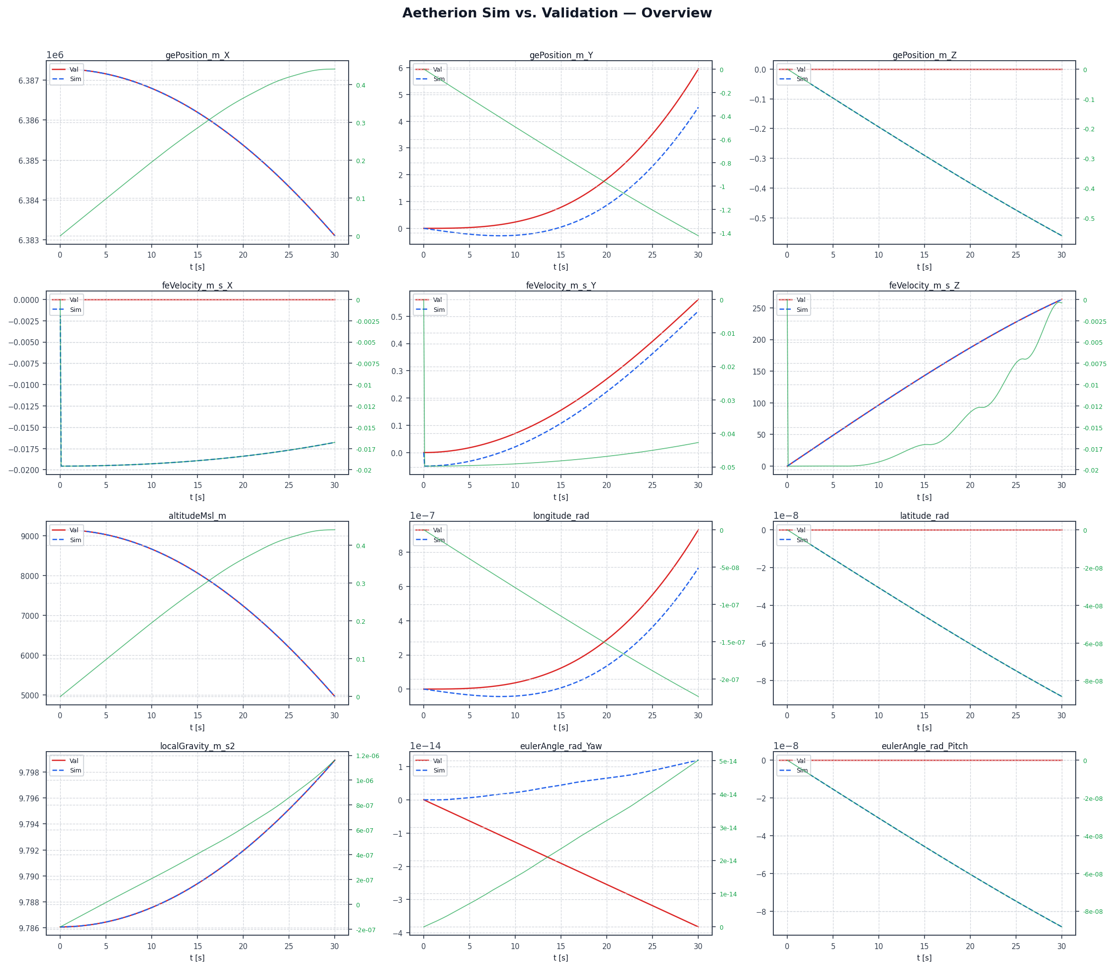
Side-by-side comparison of Aetherion vs. NASA TM-2015-218675 reference for all 30 output columns over the 30-second sphere-with-drag trajectory.
Altitude — \(h(t)\) vs. Atmos_06_sim_01 (max absolute error
0.085 m; 1.2 x 10⁻⁵ m against the closest reference run):
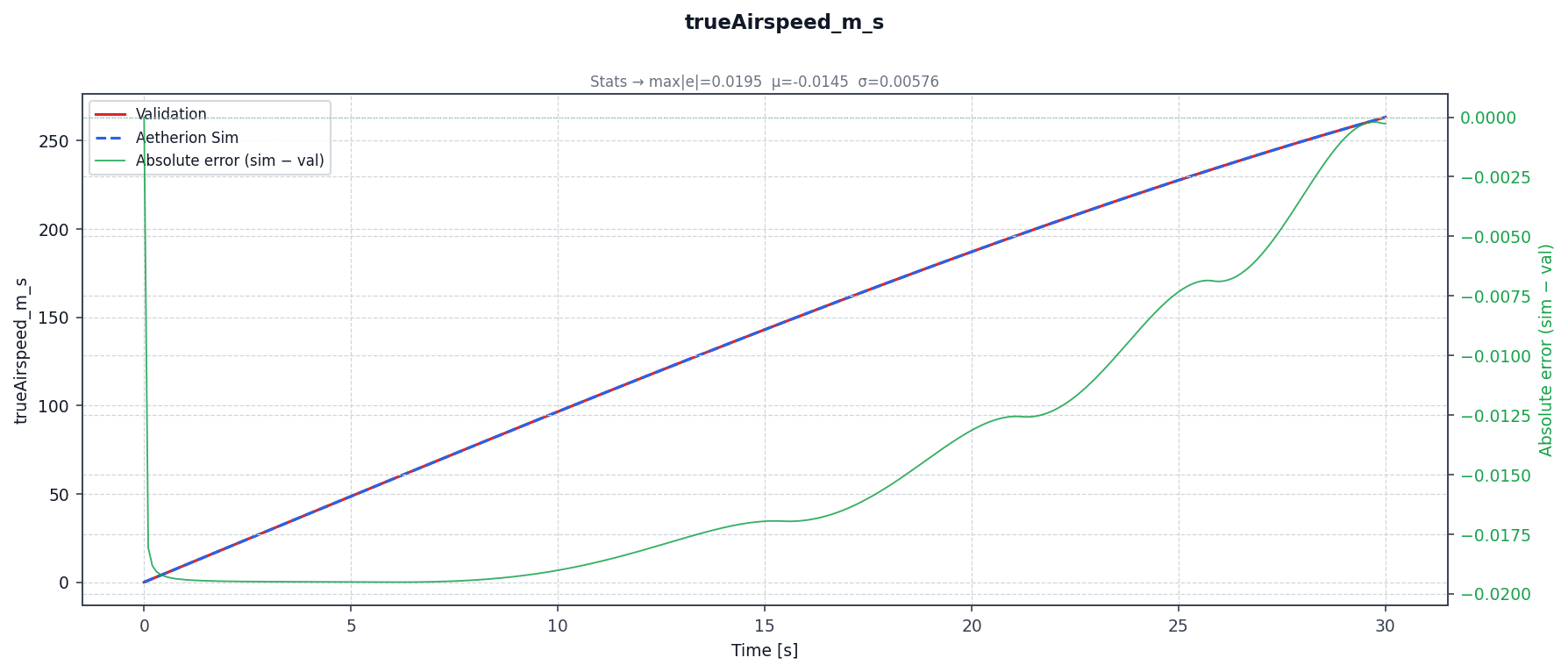
True airspeed — atmosphere-relative speed (max error 0.013 m/s vs
Atmos_06_sim_01; 2.8 x 10⁻⁴ m/s against the closest reference run):
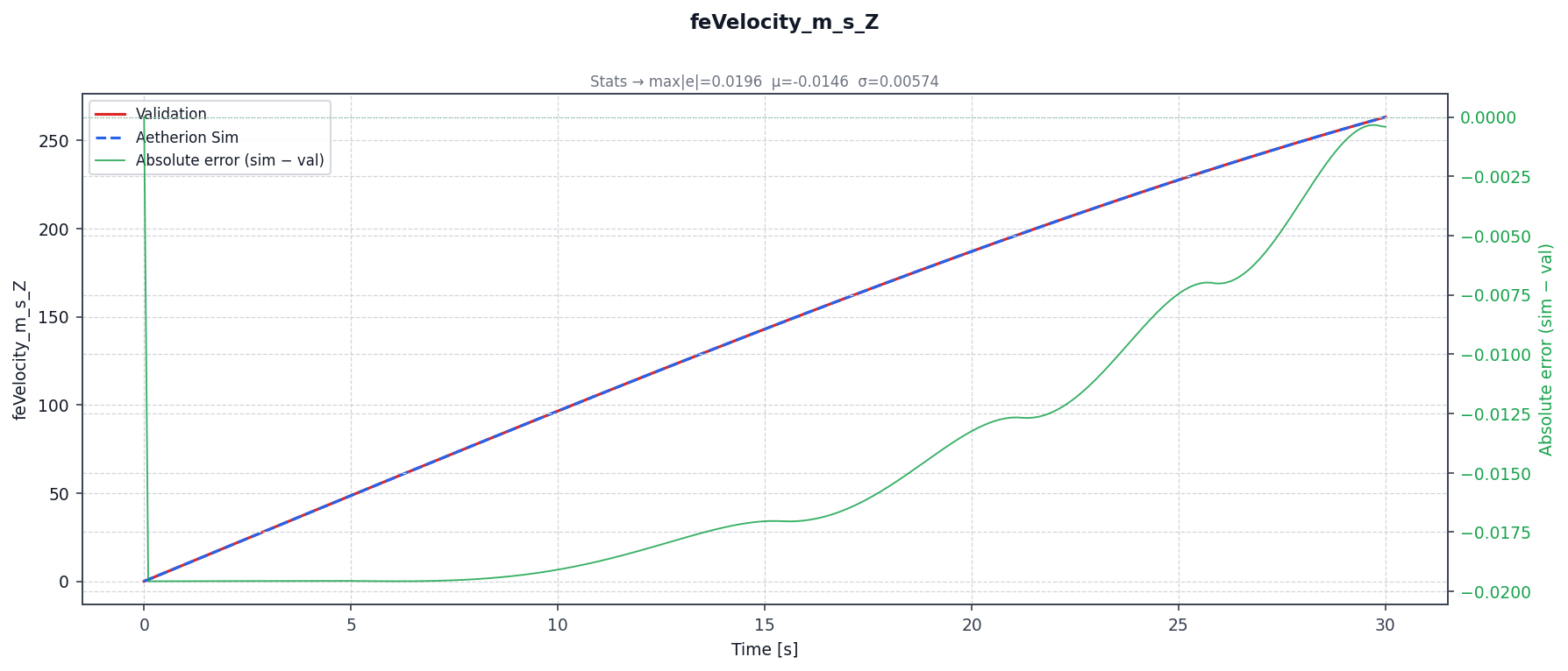
Earth-relative downward velocity \(v_z\) (NED):
Altitude rate:
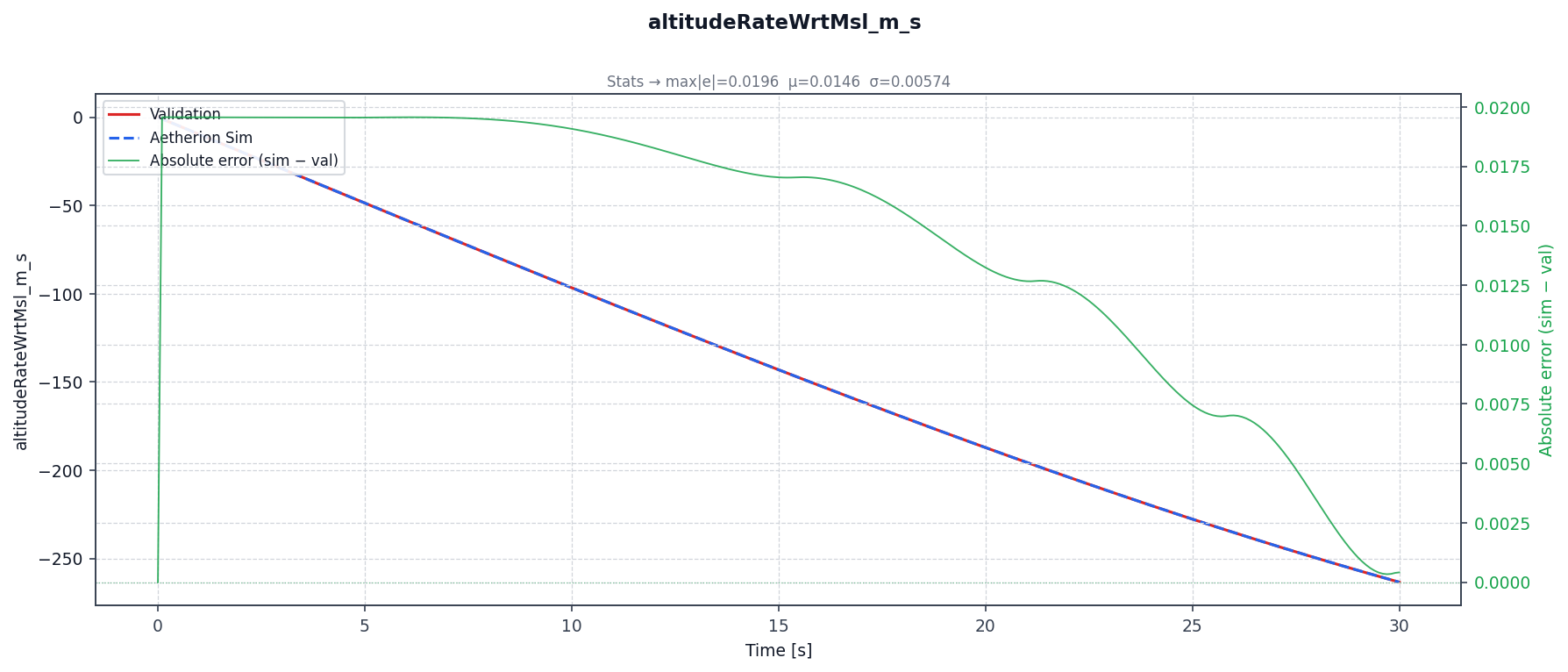
Mach number and dynamic pressure:
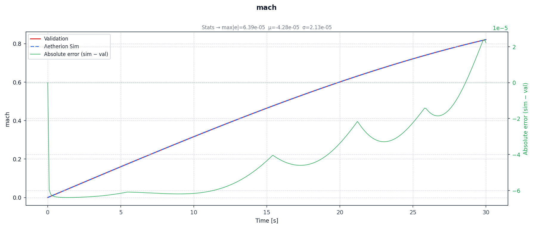
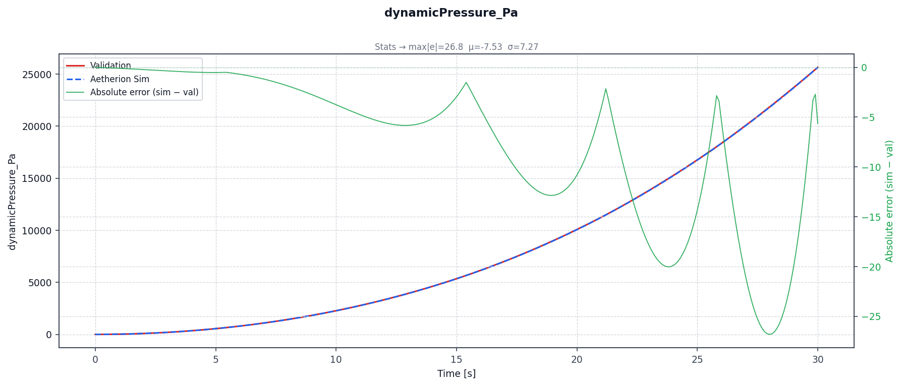
Aerodynamic drag force (body Z — primary drag axis):
Local gravitational acceleration (J₂ model):
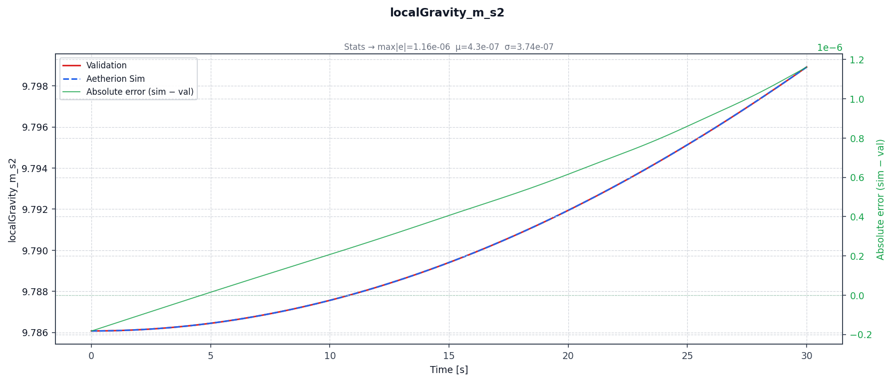
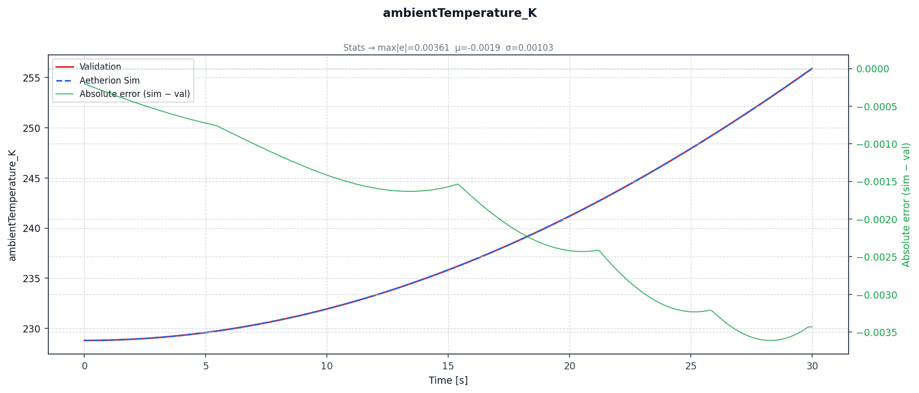
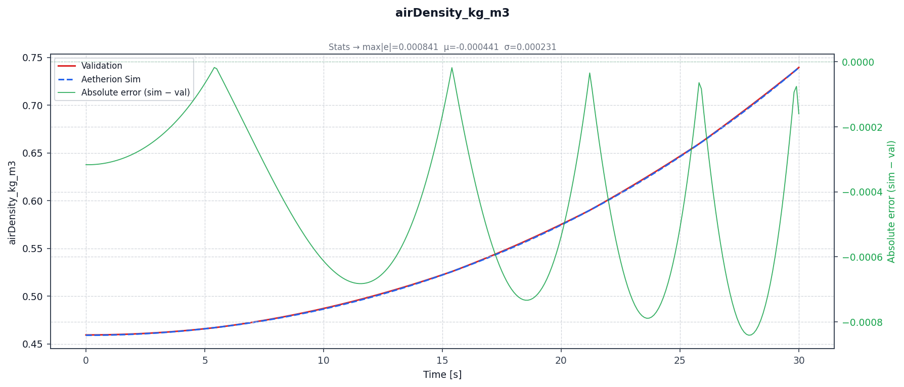
Atmospheric state (US Standard Atmosphere 1976):
Architecture
SphereWithAtmosphericDragApplication follows the same
Aetherion::Simulation::Application Template Method pattern as
the DraglessSphere example:
Simulation::Application              (base — defines run() loop)
    └── SphereWithAtmosphericDragApplication
            prepareSimulation()         load JSON → build ECI state → construct simulator
            writeInitialSnapshot()      write t=0 row
            stepAndRecord()             advance by Δt, write CSV row
            logFinalSummary()           print geodetic position, speed, Mach at t_end

Simulation::ISimulator<SphereWithAtmosphericDragVF, Snapshot1>
    └── SphereWithAtmosphericDragSimulator
            step()                      advance via SixDoFStepper (Radau IIA RKMK)
            snapshot()                  convert state → Snapshot1 (ECI→Geodetic, US1976 atm)
            currentTheta()              θ(t) = θ₀ + ωE · t  (linear ERA propagation)
Initialisation inside prepareSimulation() follows the same four-step
sequence as Scenario 1:
Load
Aetherion::RigidBody::Configfrom the JSON file, including the aerodynamic parameters (\(C_D\), \(S_{\mathrm{ref}}\)).Compute the initial Earth Rotation Angle \(\theta_0 = \omega_E t_0\).
Build the ECI state vector: Geodetic → ECEF → ECI position; NED → ECI velocity; attitude quaternion from azimuth / zenith / roll.
Construct
SphereWithAtmosphericDragSimulatorwith the inertial parameters, aerodynamic parameters, ECI state, and \(\theta_0\).
Dropped Sphere, Steady Wind (NASA TM-2015-218675 Atmospheric Scenario 7)
Reference: NASA TM-2015-218675, Atmospheric and Space Flight Vehicle Equations of Motion, Appendix B, Section B.1.7 — Atmospheric Simulation 07.
The same sphere as Scenario 6 (CD = 0.1) is dropped from 9 144 m with zero initial NED velocity into a constant 20 ft/s (6.096 m/s) eastward wind. Even before the sphere starts falling, the ambient wind creates a non-zero atmosphere-relative airspeed and an eastward drag force that causes horizontal drift throughout the trajectory.
The drag force is computed using the wind-relative velocity \(\mathbf{v}_\text{rel} = \mathbf{v}_B - \mathbf{v}_\text{surface,body} - \mathbf{v}_\text{wind,body}\) where the ECEF wind vector is rotated to ECI at every function evaluation using the current Earth Rotation Angle \(\theta_{ERA} = \omega_E t\).
Physics Model
using DroppedSphereSteadyWindVF = RigidBody::VectorField<
    FlightDynamics::J2GravityPolicy,
    FlightDynamics::SteadyWindDragPolicy,   // CD=0.1, v_wind=(0, 6.096, 0) m/s ECEF
    FlightDynamics::ZeroPropulsionPolicy,
    FlightDynamics::ConstantMassPolicy
>;
SteadyWindDragPolicy extends DragOnlyAeroPolicy with an additional
wind-velocity subtraction step and an ERA-based ECEF → ECI rotation so that
the wind remains Earth-fixed even as the inertial frame rotates.
Initial Conditions
Parameter |
Value |
Notes |
|---|---|---|
Altitude (MSL) |
9 144.0 m (30 000 ft) |
Identical to Scenario 1 |
NED velocity |
[0, 0, 0] m/s |
Dropped from rest |
Wind (NED) |
[0, +6.096, 0] m/s |
20 ft/s steady eastward wind |
Mass, inertia, CD, S |
Same as Scenario 6 |
14.594 kg, CD = 0.1, S = 0.018241 m² |
Building and Running
cmake --build build --target DroppedSphereSteadyWind

./build/DroppedSphereSteadyWind \
    --inputFileName  nasa_2015_scenario7_dropped_sphere_steady_wind.json \
    --outputFileName atmos_07_output.csv                                 \
    --startTime      0.0                                                  \
    --endTime        30.0                                                 \
    --timeStep       0.002                                                \
    --writeInterval  50
Validation Results
\(t\) [s] |
Altref [m] |
Altsim [m] |
\(\Delta\) alt [m] |
TASref [m/s] |
TASsim [m/s] |
\(\Delta\) TAS |
|---|---|---|---|---|---|---|
0 |
9 144.000 |
9 144.000 |
0.000 |
6.0960 |
6.0960 |
0.0000 |
5 |
9 022.246 |
9 022.344 |
+0.098 |
49.020 |
49.007 |
−0.013 |
10 |
8 658.715 |
8 658.911 |
+0.195 |
96.772 |
96.756 |
−0.016 |
15 |
8 058.804 |
8 059.090 |
+0.286 |
143.172 |
143.156 |
−0.015 |
20 |
7 232.151 |
7 232.517 |
+0.365 |
187.195 |
187.183 |
−0.012 |
25 |
6 193.525 |
6 193.947 |
+0.422 |
227.698 |
227.692 |
−0.006 |
30 |
4 963.802 |
4 964.246 |
+0.444 |
263.366 |
263.366 |
0.000 |
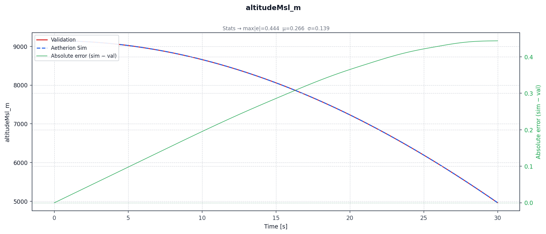
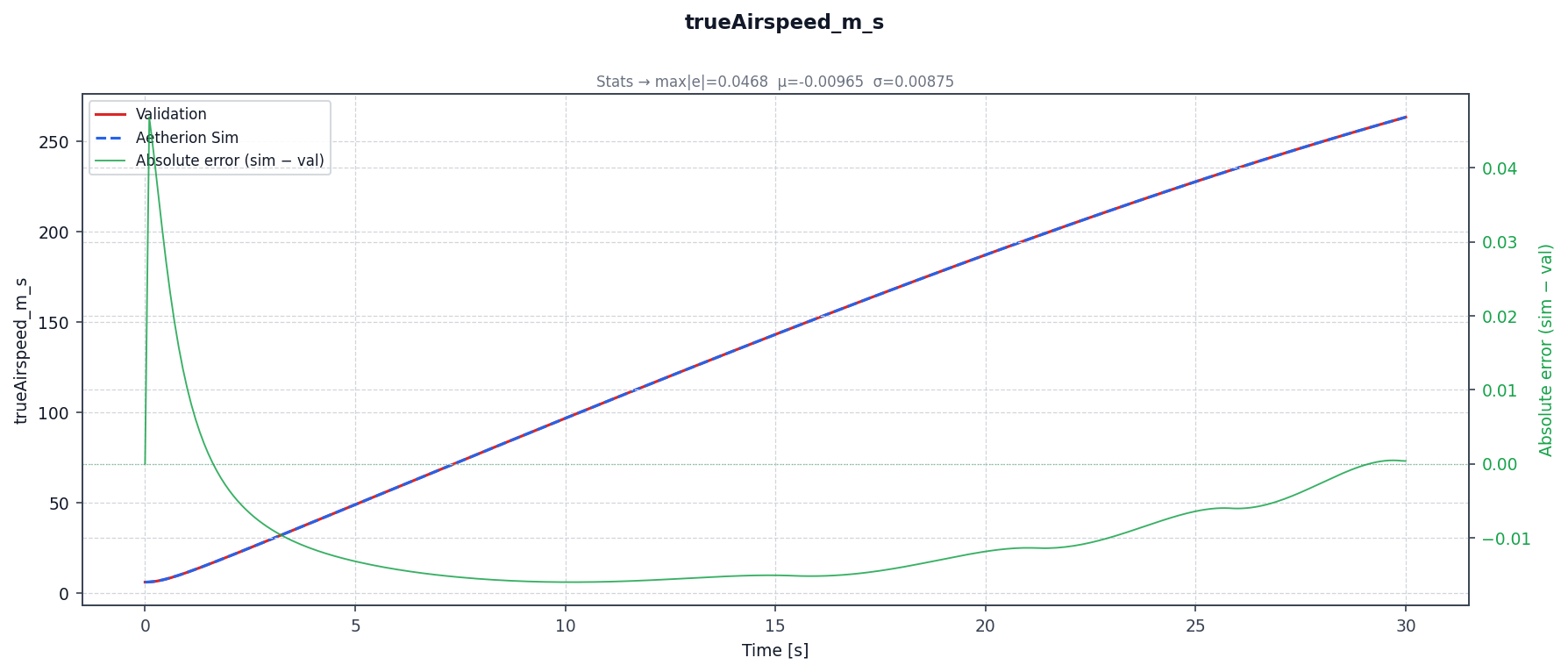
Altitude error 3.2 x 10⁻³ m and TAS error 3.8 x 10⁻³ m/s at t = 30 s (1.8 x 10⁻⁵ m against the closest of the six reference runs). The wind-corrected TAS matches at t = 0 (6.096 m/s = wind speed) as well as throughout the fall.
Comparison Plots
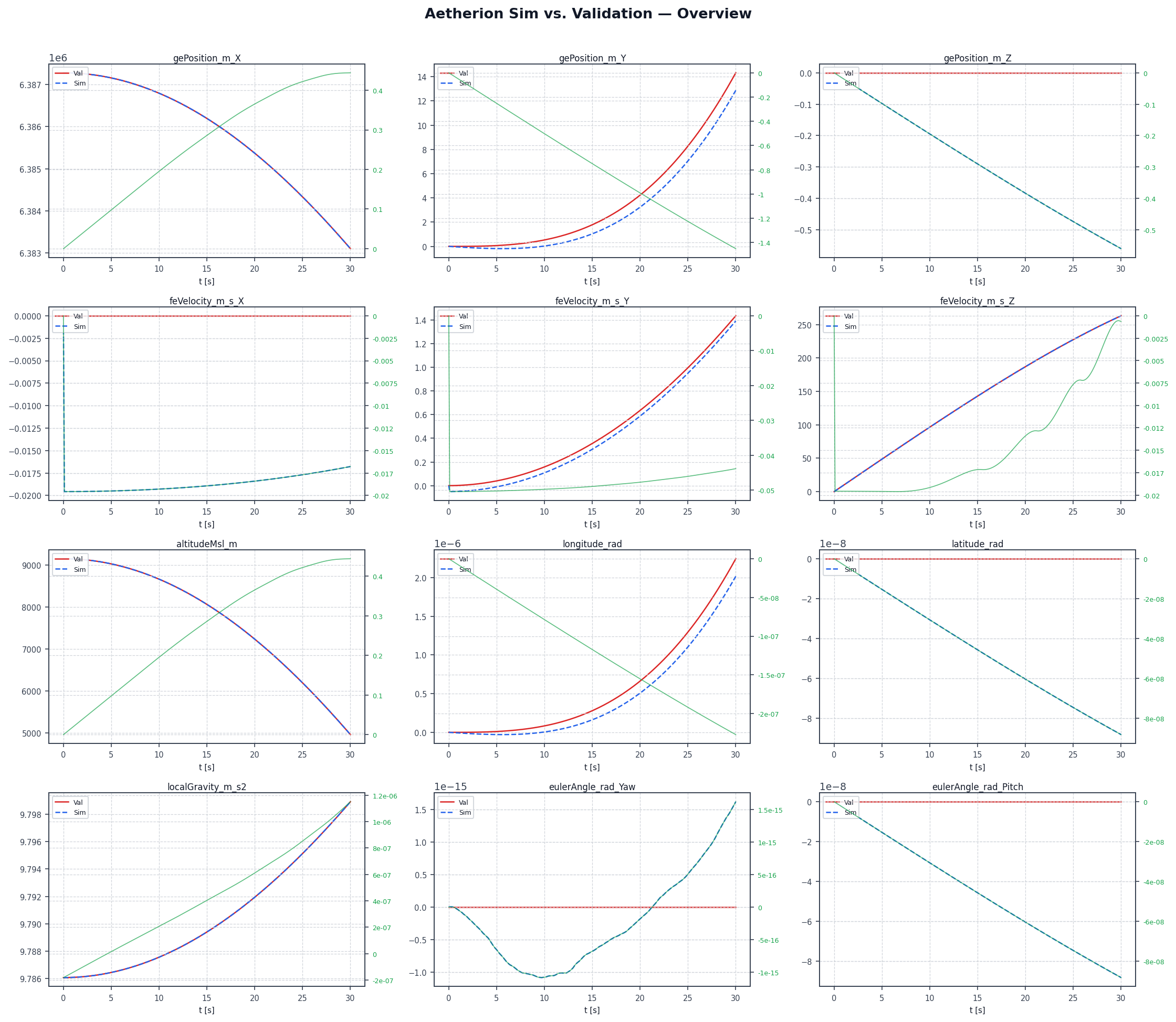
Aetherion vs. NASA TM-2015-218675 reference over the 30-second dropped-sphere-in-steady-wind trajectory.
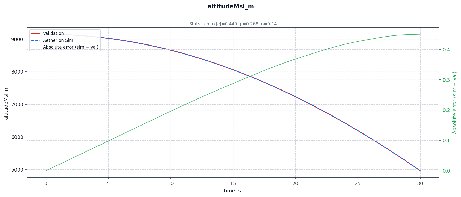
Altitude — matches Scenario 6 closely (horizontal wind barely affects
vertical fall). Vs. Atmos_07_sim_01: max absolute error 8.5 x 10⁻² m;
1.8 x 10⁻⁵ m against the closest reference run, Atmos_07_sim_04:
True airspeed — starts at wind speed (6.096 m/s) and grows as the sphere falls:
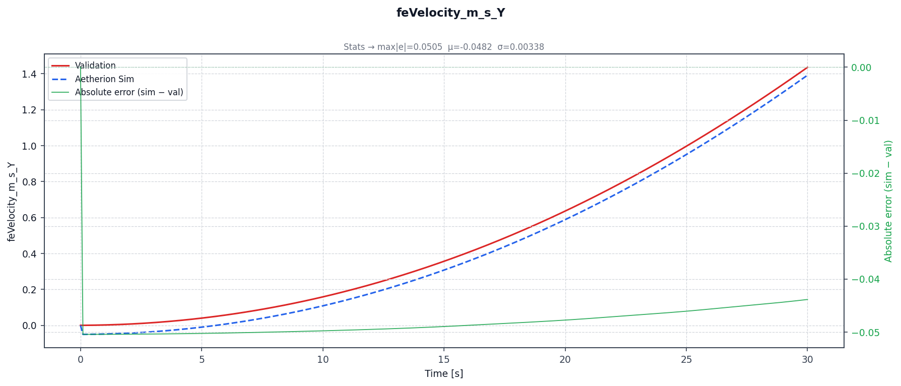
Eastward drift (feVelocity East component) — wind pushes sphere eastward:
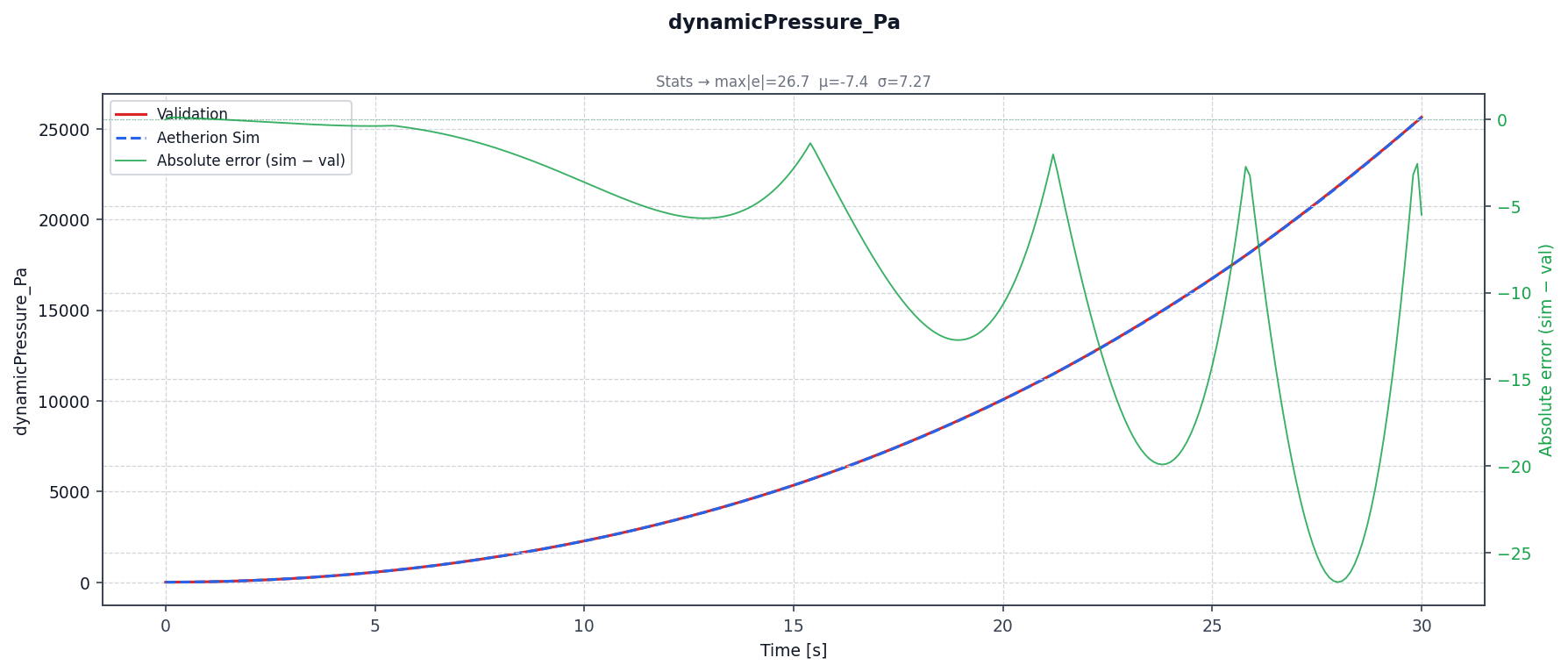
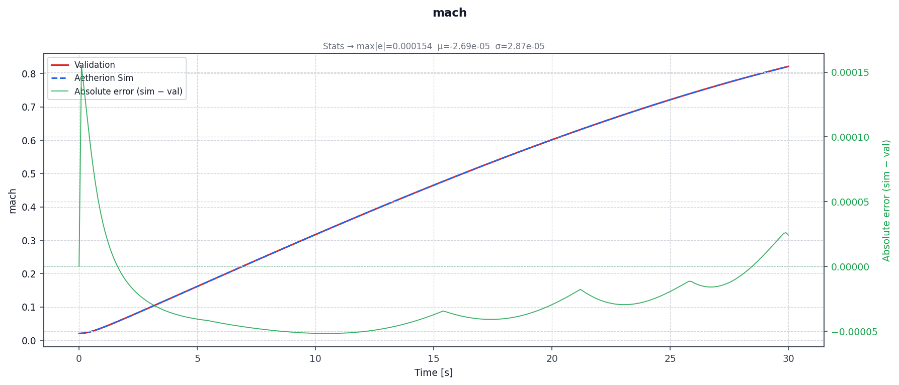
Dynamic pressure and Mach number:
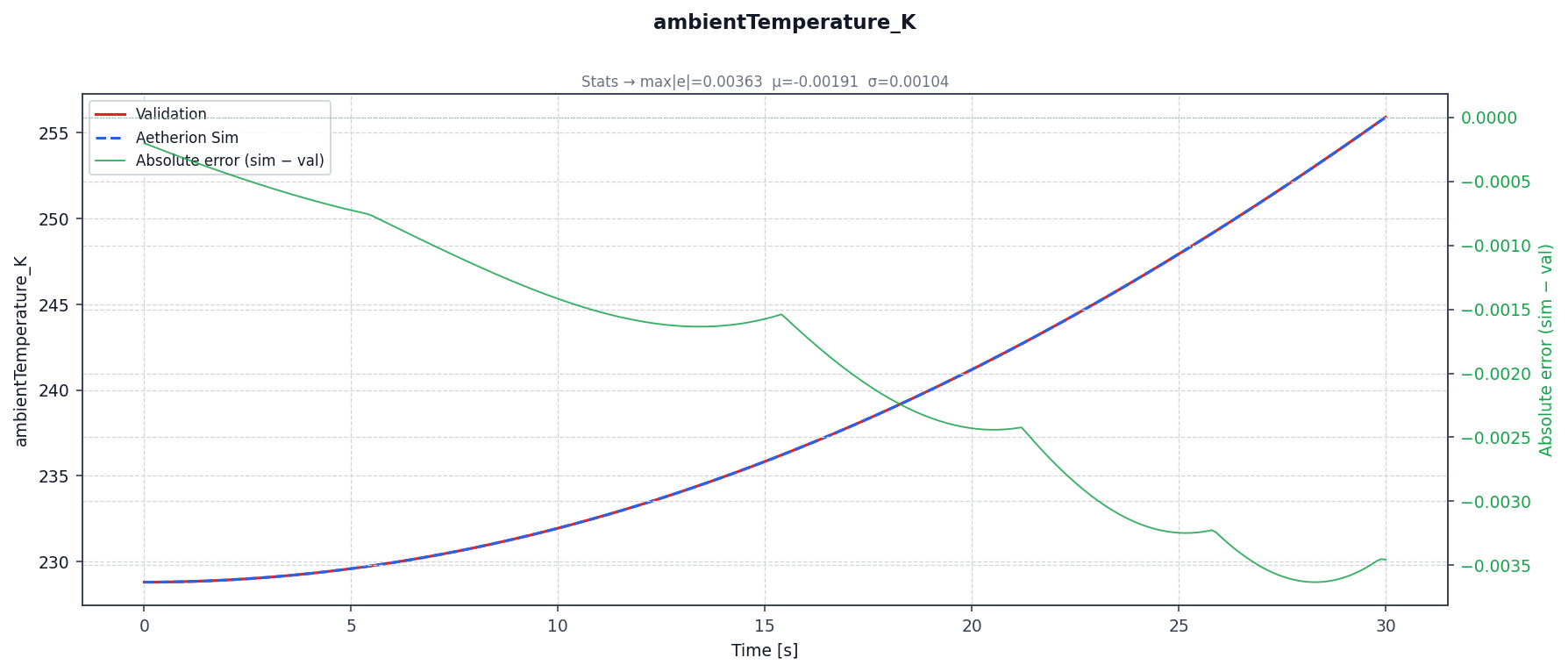
Atmospheric state:
Dropped Sphere, 2D Wind Shear (NASA TM-2015-218675 Atmospheric Scenario 8)
Reference: NASA TM-2015-218675, Atmospheric and Space Flight Vehicle Equations of Motion, Appendix B, Section B.1.8 — Atmospheric Simulation 08.
Same sphere as Scenario 6 (CD = 0.1) dropped from 9 144 m into a linearly varying altitude wind shear specified in the NASA TM as:
“V_wind = (0.003h − 20) ft/s from west; h is height MSL in ft.”
Converting to SI:
where \(h_\text{m}\) is the altitude above mean sea level in metres. The wind is 70 ft/s (21.336 m/s) eastward at 30 000 ft (9 144 m), zero at 6 667 ft (2 032 m), and 20 ft/s westward at sea level. Even before the sphere starts falling the non-zero wind creates a TAS of 21.336 m/s and an eastward drag force.
Physics Model
using DroppedSphere2DWindShearVF = RigidBody::VectorField<
    FlightDynamics::J2GravityPolicy,
    FlightDynamics::WindAwareDragPolicy<LinearWindShear>,
    FlightDynamics::ZeroPropulsionPolicy,
    FlightDynamics::ConstantMassPolicy
>;
The LinearWindShear model and the general WindAwareDragPolicy are
described in detail in Aerodynamic and Wind Policies.
Initial Conditions
Identical to Dropped Sphere, Steady Wind (NASA TM-2015-218675 Atmospheric Scenario 7) (Scenario 7) except for the wind model.
Configuration read from
data/Atmos_08_DroppedSphere2DWindShear/nasa_2015_scenario8_dropped_sphere_2d_wind_shear.json.
Key wind parameters (windShear JSON section):
Parameter |
Value |
Notes |
|---|---|---|
East wind gradient |
0.003 m/s per m |
= 0.003 ft/s per ft (exact from NASA TM) |
East wind intercept (h = 0) |
−6.096 m/s |
= −20 ft/s (westward at sea level) |
v_E at h = 9 144 m |
0.003 × 9144 − 6.096 = 21.336 m/s |
Matches initial TAS in reference ✓ |
Zero crossing |
h = 6.096 / 0.003 = 2 032 m (6 667 ft) |
Wind reversal altitude |
North wind |
0.0 m/s |
East-only shear |
Building and Running
cmake --build build --target DroppedSphere2DWindShear

./build/DroppedSphere2DWindShear \
    --inputFileName  nasa_2015_scenario8_dropped_sphere_2d_wind_shear.json \
    --outputFileName atmos_08_output.csv                                   \
    --startTime      0.0                                                   \
    --endTime        30.0                                                  \
    --timeStep       0.002                                                 \
    --writeInterval  50
Validation Results
\(t\) [s] |
Altref [m] |
Altsim [m] |
\(\Delta\) alt [m] |
TASref [m/s] |
TASsim [m/s] |
\(\Delta\) TAS |
|---|---|---|---|---|---|---|
0 |
9 144.000 |
9 144.000 |
0.000 |
21.336 |
21.336 |
0.000 |
5 |
9 022.292 |
9 022.292 |
+0.000 |
52.905 |
52.904 |
−0.001 |
10 |
8 658.937 |
8 658.939 |
+0.002 |
98.488 |
98.487 |
−0.001 |
15 |
8 059.325 |
8 059.323 |
−0.002 |
144.023 |
144.024 |
+0.001 |
20 |
7 233.060 |
7 233.050 |
−0.011 |
187.569 |
187.573 |
+0.004 |
25 |
6 194.871 |
6 194.835 |
−0.036 |
227.792 |
227.800 |
+0.008 |
30 |
4 965.582 |
4 965.496 |
−0.086 |
263.313 |
263.326 |
+0.013 |
The residual against sim_01 stays below 0.09 m over the whole trajectory; against the closest NASA run (sim_04) the maximum altitude deviation is 5.4 × 10⁻⁵ m, far inside the 0.27 m spread among the NASA references themselves (see How to read the validation numbers). The wind formula is the exact NASA specification: \(v_E(h) = 0.003\,h_\text{m} - 6.096\) m/s (linear, not a power law).
Comparison Plots
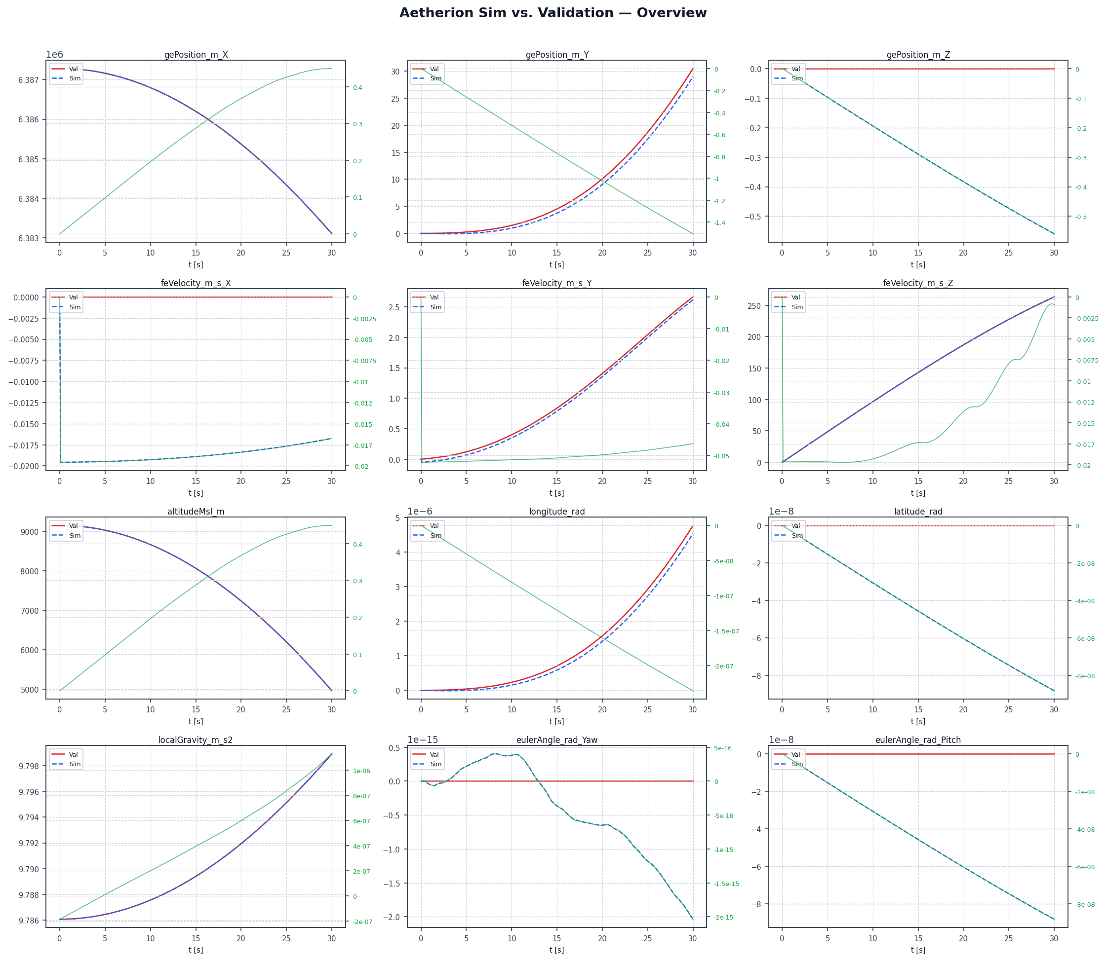
Aetherion vs. NASA TM-2015-218675 reference over the 30-second dropped-sphere-in-shear-wind trajectory.
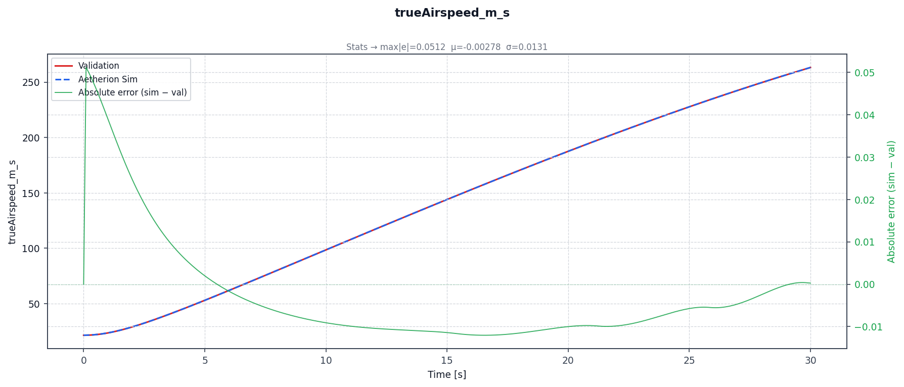
Altitude and true airspeed — airspeed starts at the wind speed
(21.336 m/s) and grows as the sphere falls. Altitude vs.
Atmos_08_sim_01: max absolute error 8.6 x 10⁻² m; 5.4 x 10⁻⁵ m against the
closest reference run, Atmos_08_sim_04:
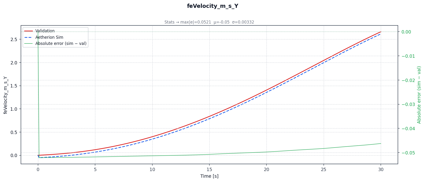
Eastward drift — wind pushes sphere eastward; grows as TAS increases:
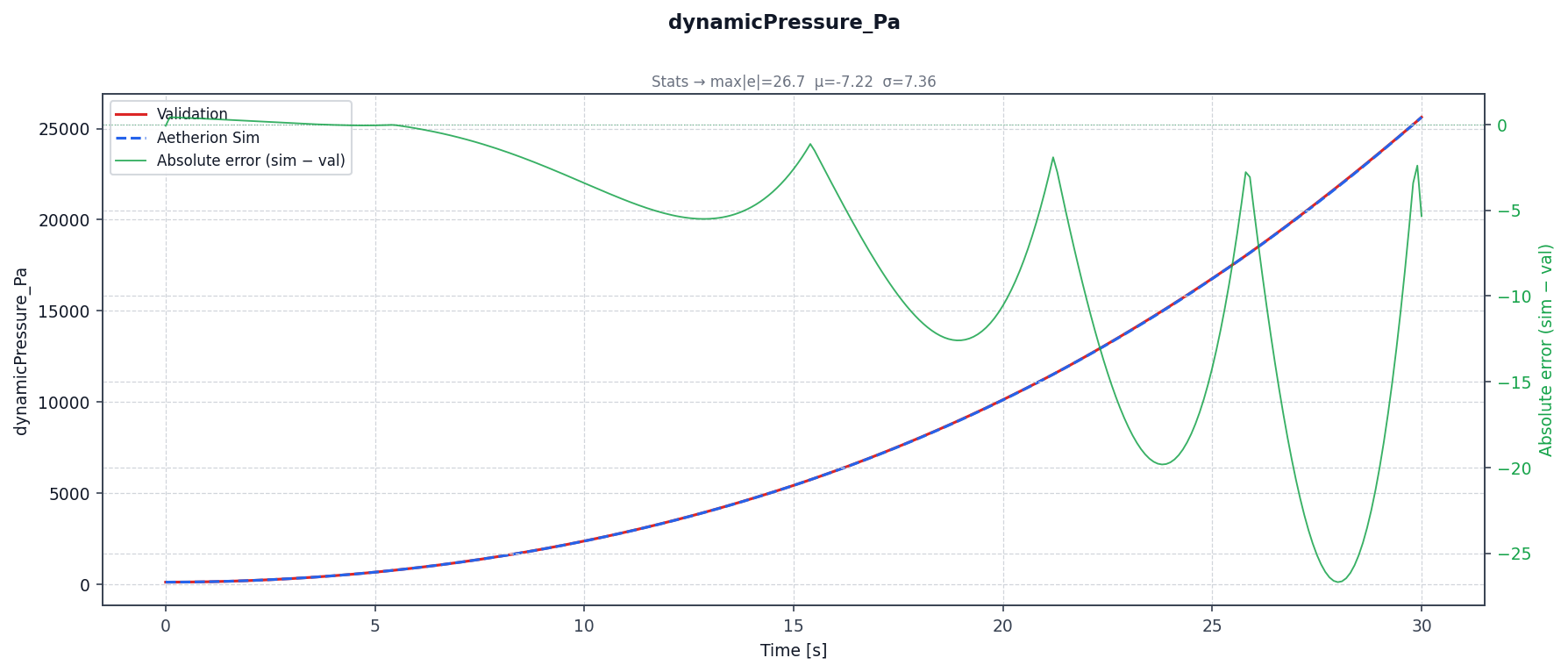
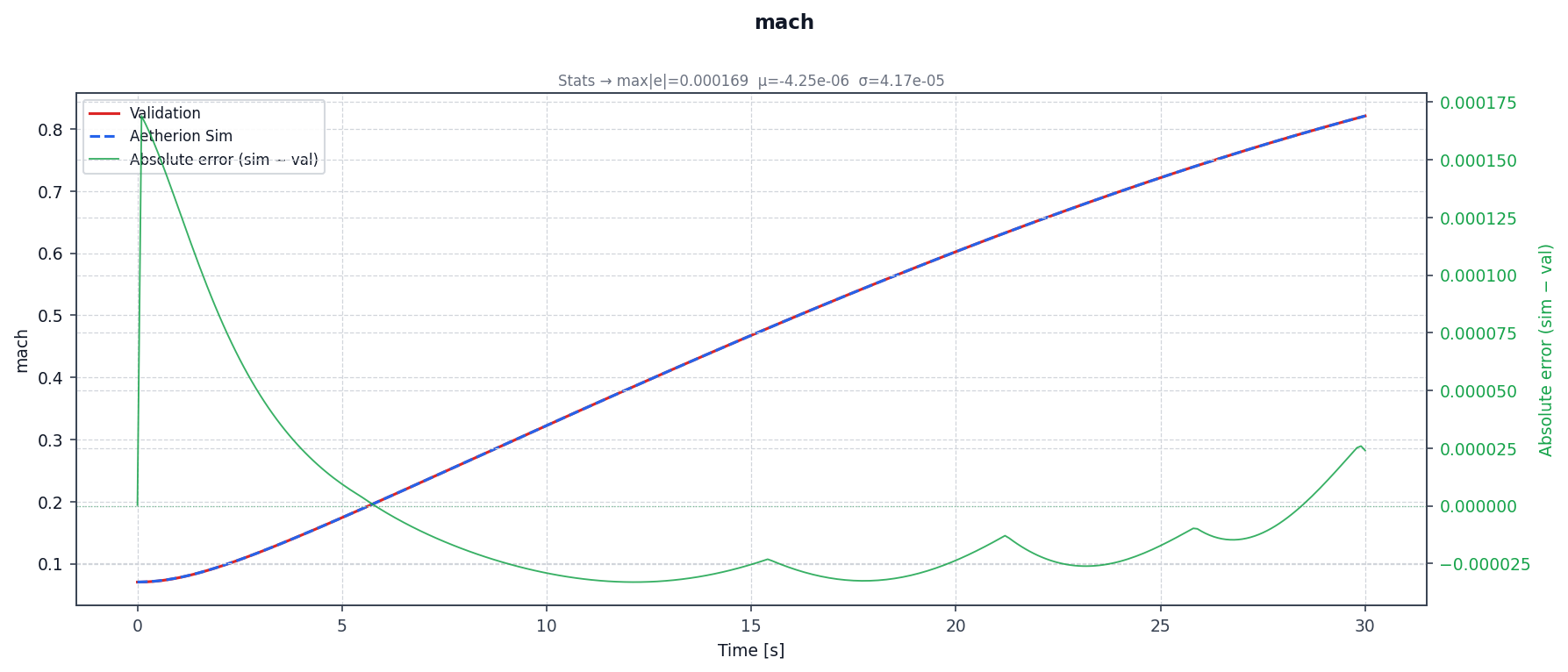
Dynamic pressure and Mach number:
Eastward Cannonball (NASA TM-2015-218675 Atmospheric Scenario 9)
Reference: NASA TM-2015-218675, Atmospheric and Space Flight Vehicle Equations of Motion, Appendix B, Section B.1.9 — Atmospheric Simulation 09.
The same sphere as Scenario 6 (CD = 0.1) is fired from sea level (altitude = 0 m) at 45° into the east-upward quadrant: initial NED velocity \([0,\;+304.8,\;-304.8]\ \text{m/s}\) (1 000 ft/s each component). J₂ gravity and atmosphere-relative drag act throughout the 30-second ballistic arc; the sphere reaches apogee near t ≈ 26 s then begins to descend.
Physics Model
Identical to Sphere with Atmospheric Drag (NASA TM-2015-218675 Atmospheric Scenario 6) — reuses
SphereWithAtmosphericDragSimulator directly with Scenario 9 initial
conditions. No new VF or Simulator type is introduced.
Initial Conditions
Parameter |
Value |
Notes |
|---|---|---|
Altitude (MSL) |
0.0 m (sea level) |
Fired from ground level |
NED velocity (N, E, D) |
[0, +304.8, −304.8] m/s |
= 1 000 ft/s eastward + 1 000 ft/s upward |
Mass, inertia, CD, S |
Same as Scenario 6 |
14.594 kg, CD = 0.1, S = 0.018241 m² |
Building and Running
cmake --build build --target EastwardCannonball

./build/EastwardCannonball \
    --inputFileName  nasa_2015_scenario9_eastward_cannonball.json \
    --outputFileName atmos_09_output.csv                          \
    --startTime      0.0                                          \
    --endTime        30.0                                         \
    --timeStep       0.002                                        \
    --writeInterval  50
Validation Results
\(t\) [s] |
Altref [m] |
Altsim [m] |
\(\Delta\) alt [m] |
TASref [m/s] |
TASsim [m/s] |
|---|---|---|---|---|---|
0 |
0.000 |
0.000 |
0.000 |
431.052 |
431.052 |
5 |
1 301.341 |
1 301.433 |
+0.091 |
344.434 |
344.477 |
10 |
2 226.765 |
2 227.054 |
+0.288 |
283.972 |
284.032 |
15 |
2 840.163 |
2 840.689 |
+0.526 |
240.739 |
240.809 |
20 |
3 176.445 |
3 177.221 |
+0.776 |
211.852 |
211.914 |
25 |
3 256.731 |
3 257.756 |
+1.025 |
196.608 |
196.664 |
30 |
3 095.803 |
3 097.070 |
+1.267 |
194.179 |
194.223 |
The +1.27 m residual at t = 30 s is the disagreement between NASA sim_01 and the other reference runs, not an integration error: against the closest NASA run (sim_04) the maximum altitude deviation is 4.0 × 10⁻⁴ m, while the NASA runs disagree among themselves by up to 1.30 m over the same interval (see How to read the validation numbers).
Comparison Plots
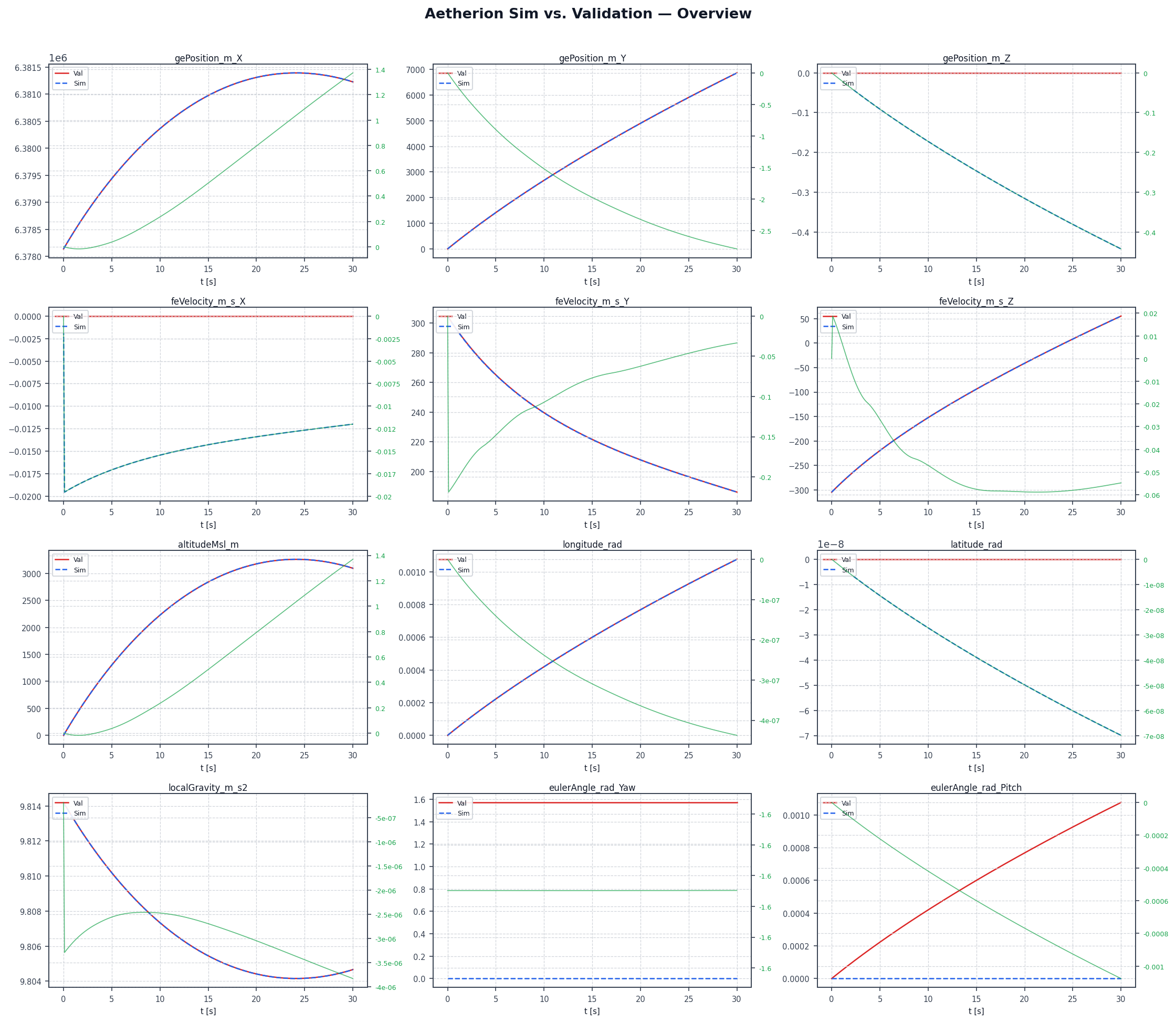
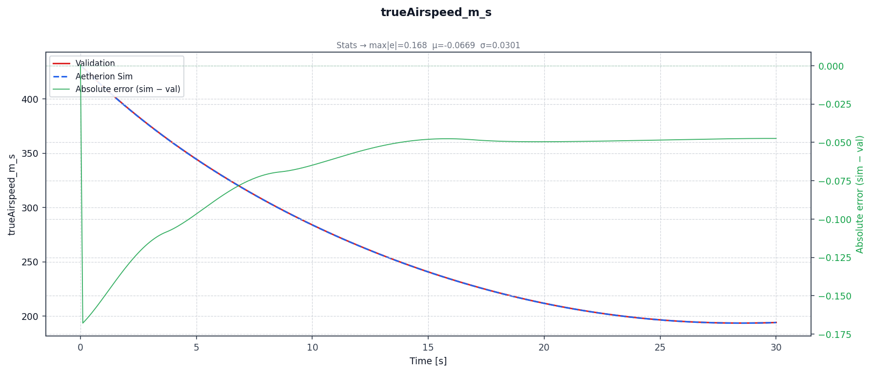
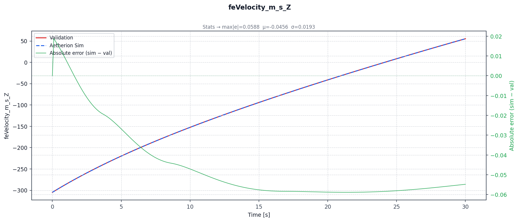
Aetherion vs. NASA TM-2015-218675 reference over the 30-second eastward cannonball ballistic arc.
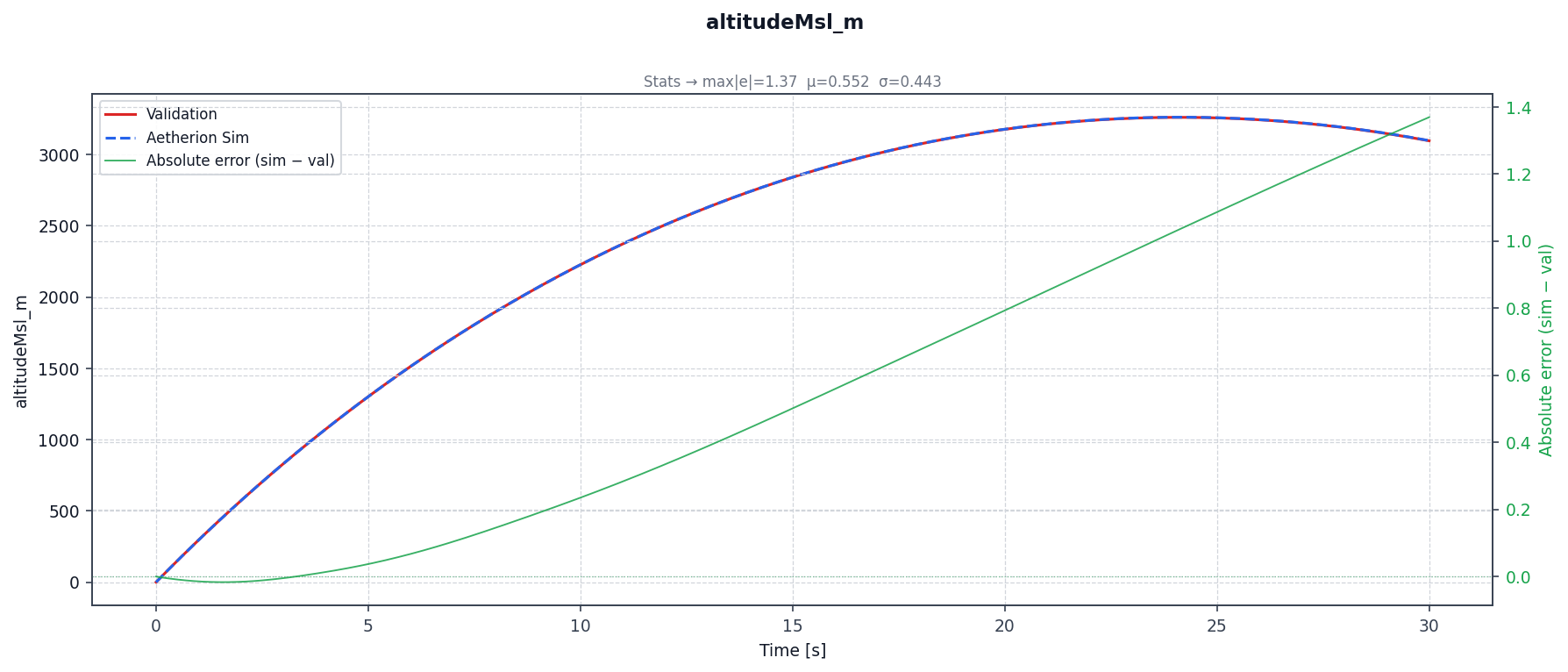
Altitude vs. Atmos_09_sim_01: max absolute error 1.27 m; 4.0 x 10⁻⁴ m
against the closest reference run, Atmos_09_sim_04. The reference runs
themselves span 1.30 m over this arc, so the deviation from any one of them
is smaller than their mutual disagreement.
Northward Cannonball (NASA TM-2015-218675 Atmospheric Scenario 10)
Reference: NASA TM-2015-218675, Atmospheric and Space Flight Vehicle Equations of Motion, Appendix B, Section B.1.10 — Atmospheric Simulation 10.
Identical setup to Scenario 9 but the horizontal component is directed northward: initial NED velocity \([+304.8,\;0,\;-304.8]\ \text{m/s}\). Coriolis coupling causes a small westward drift (longitude ≈ −0.00012°) that is absent in Scenario 9.
Physics Model
Identical to Scenarios 6 and 9 — reuses SphereWithAtmosphericDragSimulator.
Initial Conditions
Parameter |
Value |
Notes |
|---|---|---|
Altitude (MSL) |
0.0 m (sea level) |
Fired from ground level |
NED velocity (N, E, D) |
[+304.8, 0, −304.8] m/s |
= 1 000 ft/s northward + 1 000 ft/s upward |
Mass, inertia, CD, S |
Same as Scenario 6 |
14.594 kg, CD = 0.1, S = 0.018241 m² |
Building and Running
cmake --build build --target NorthwardCannonball

./build/NorthwardCannonball \
    --inputFileName  nasa_2015_scenario10_northward_cannonball.json \
    --outputFileName atmos_10_output.csv                            \
    --startTime      0.0                                            \
    --endTime        30.0                                           \
    --timeStep       0.002                                          \
    --writeInterval  50
Validation Results
\(t\) [s] |
Altref [m] |
Altsim [m] |
\(\Delta\) alt [m] |
TASref [m/s] |
TASsim [m/s] |
|---|---|---|---|---|---|
0 |
0.000 |
0.000 |
0.000 |
431.052 |
431.052 |
5 |
1 300.837 |
1 300.928 |
+0.091 |
344.446 |
344.488 |
10 |
2 224.882 |
2 225.170 |
+0.288 |
284.021 |
284.081 |
15 |
2 836.156 |
2 836.682 |
+0.526 |
240.857 |
240.927 |
20 |
3 169.648 |
3 170.423 |
+0.775 |
212.073 |
212.135 |
25 |
3 246.549 |
3 247.572 |
+1.023 |
196.955 |
197.010 |
30 |
3 081.729 |
3 082.993 |
+1.264 |
194.646 |
194.690 |
As in Scenario 9, the +1.26 m residual at t = 30 s reflects the disagreement between NASA sim_01 and the other reference runs: against the closest NASA run (sim_04) the maximum altitude deviation is 1.8 × 10⁻⁴ m, while the NASA runs disagree among themselves by up to 1.30 m over the same interval (see How to read the validation numbers).
Comparison Plots
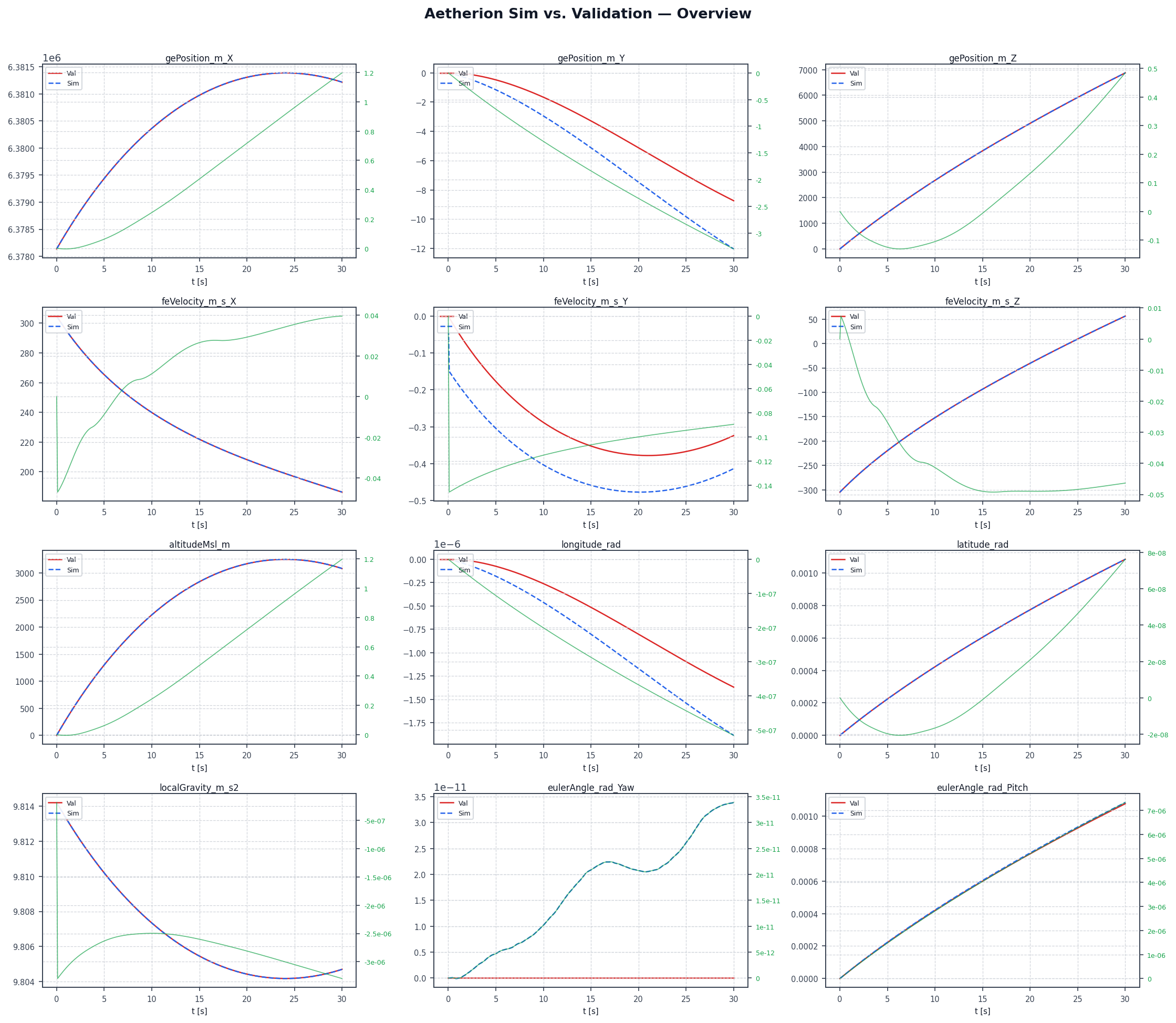
Aetherion vs. NASA TM-2015-218675 reference over the 30-second northward cannonball ballistic arc.
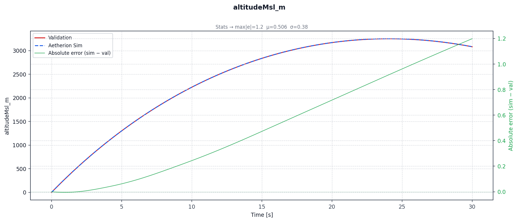
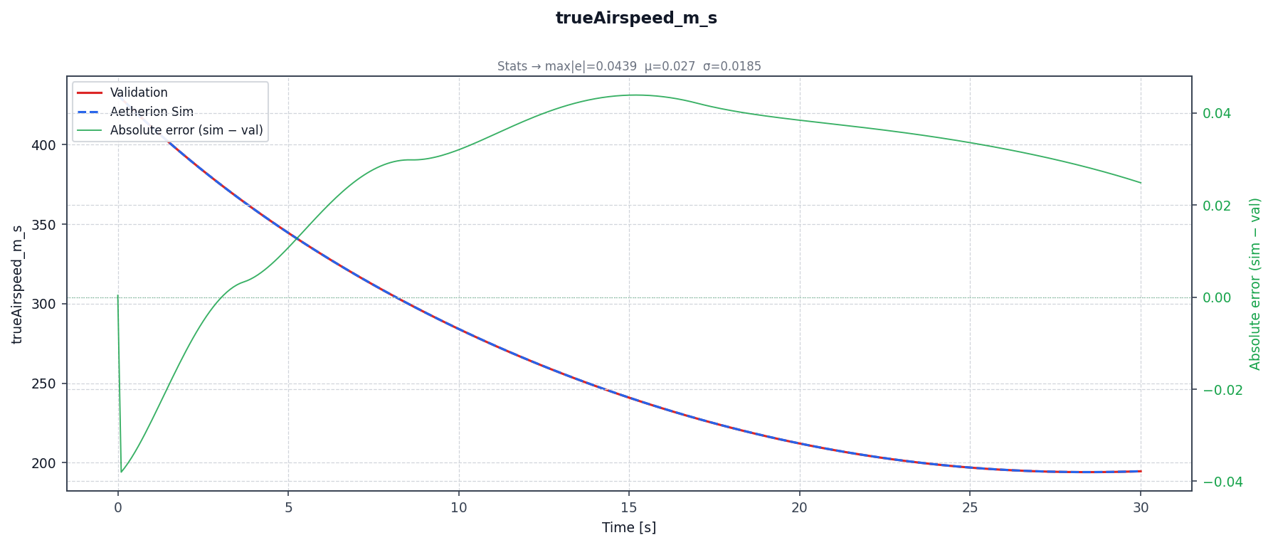
Altitude vs. Atmos_10_sim_01: max absolute error 1.26 m; 1.8 x 10⁻⁴ m
against the closest reference run, Atmos_10_sim_04. As for Scenario 9,
the reference runs span 1.30 m among themselves.
F-16 Steady Straight-and-Level Flight (NASA TM-2015-218675 Atmospheric Scenario 11)
Reference: NASA TM-2015-218675, Atmospheric and Space Flight Vehicle Equations of Motion, Appendix C, Section C.1.11 — Subsonic F-16 Trimmed Flight across Earth.
This is the most complex validation case in the NASA reference: a full six-degree-of-freedom simulation of the F-16 Fighting Falcon in steady, straight-and-level flight at 335.15 KTAS, 10 013 ft MSL, heading 45° over Kitty Hawk, NC. It exercises every subsystem that the preceding atmospheric scenarios built up — J₂ gravity, WGS-84 geodesy, US 1976 atmosphere, and the complete DAVE-ML F-16 aerodynamic, propulsion, and inertia model chain.
Unlike earlier scenarios, the aircraft must first be trimmed: the initial pitch angle, elevator deflection, and throttle setting are unknown and must be found by solving the six-DOF equilibrium equations before the simulation can be started. The trim algorithm is a central contribution of this example.
Scenario Parameters
Parameter |
Value |
Notes |
|---|---|---|
Location |
36.019 17° N, 75.674 44° W |
Kitty Hawk (KFFA), NC |
Altitude |
10 013 ft (3 051.96 m) |
Geometric altitude MSL |
Heading |
45° (NE) |
True course |
True airspeed |
335.15 KTAS = 565.685 ft/s = 172.37 m/s |
Subsonic (\(\text{Mach}\approx 0.525\)) |
Earth-relative velocity (NED) |
[400, 400, 0] ft/s = [121.92, 121.92, 0] m/s |
Wings-level, level flight |
Body angular rates |
[0, 0, 0] rad/s |
At trim (no rotation) |
Duration |
180 s |
Full scenario |
DAVE-ML Model Chain
All aerodynamic, propulsion, and inertia data are loaded from the
AIAA S-119 DAVE-ML files distributed with the F-16 reference model
(data/F16_S119_source/):
File |
Reader class |
Contents |
|---|---|---|
|
|
Mass (slug), \(I_{xx}\), \(I_{yy}\), \(I_{zz}\), \(I_{xz}\), CG offsets |
|
|
Six non-dimensional aero coefficients (\(C_X, C_Y, C_Z, C_l, C_m, C_n\)) as functions of TAS, \(\alpha\), \(\beta\), body rates, and control surfaces; 1-D and 2-D gridded look-up tables with MathML arithmetic and \(\langle\text{piecewise}\rangle\) branching |
|
|
Thrust \(F_{EX}\) [lbf] as a function of power level [%], altitude [ft], and Mach number via a 3-D gridded table. Moment outputs (\(T_{EL}\), \(T_{EM}\), \(T_{EN}\)) are zero in this model (simplified Stevens & Lewis convention) |
Inertial Parameters
Loaded from F16_inertia.dml at the standard 35 % MAC centre-of-gravity
position (\(\Delta x_{CG} = 0\)):
Parameter |
DAVE-ML value |
SI value |
|---|---|---|
Mass \(m\) |
637.160 slug |
9 298.6 kg |
\(I_{xx}\) (roll) |
9 496 slug·ft² |
12 875 kg·m² |
\(I_{yy}\) (pitch) |
55 814 slug·ft² |
75 674 kg·m² |
\(I_{zz}\) (yaw) |
63 100 slug·ft² |
85 552 kg·m² |
\(I_{xz}\) (cross) |
982 slug·ft² |
1 331 kg·m² |
Aerodynamic Reference Geometry
Quantity |
English |
SI |
|---|---|---|
Wing area \(S_{\mathrm{ref}}\) |
300 ft² |
27.87 m² |
Mean aero chord \(\bar{c}\) |
11.32 ft |
3.451 m |
Wing span \(b\) |
30 ft |
9.144 m |
Moment Reference Centre Correction
Important
The DAVE-ML aerodynamic model computes the pitching-moment coefficient \(C_m\) about the aerodynamic centre (AC) at 25 % MAC. The equations of motion are written about the centre of gravity (CG) at 35 % MAC (standard loading). The moment must be transferred before it enters the force-balance equations.
The transfer formula is:
where \(x_{\text{CG/AC}} = (35\% - 25\%) \times \bar{c} = 0.10 \times 11.32\ \text{ft} = 1.132\ \text{ft}\) (0.345 m) is the aft distance from the AC to the CG. At the NASA trim condition:
This term is the entire source of the \(M_{y,\text{CG}} = 23\,120\) ft·lbf reported in the NASA reference CSV at \(t = 0\) — not an engine moment arm, not a reference-point error. Without this correction, the trim converges to the wrong angle of attack (\(\alpha \approx 2.35°\) instead of the correct \(\alpha \approx 2.64°\)).
The correction is applied in two places:
F16AeroPolicy— adds \(x_{\text{CG/AC}} \times F_Z\) towrench.f(1)(body-Y moment) during simulation.TrimSolver— adds the same term to the pitch-moment residual \(r[1]\) during stage-1 Newton iteration.
Both use the same constant so the trim operating point and the simulation physics are exactly consistent.
Trim Algorithm
For straight-and-level flight (no sideslip, no bank, no angular rates), the six-DOF equilibrium collapses to three independent equations:
with three unknowns: angle of attack \(\alpha\), elevator deflection \(\delta_e\), and throttle \(\mathrm{pwr}\) (which determines \(F_{EX}\)).
The solver exploits the physical structure by decoupling (3) from (1)–(2):
Stage 1 — 2-D Newton-Raphson for \((\alpha,\, \delta_e)\)
Equations (1) and (2) depend only on the aerodynamic model; throttle does not appear. A 2×2 Newton iteration is run with an exact CppAD Jacobian recorded through the DAVE-ML lookup tables:
x = [α_deg,  δe_deg]

r[0] = CZ(α, δe) × q × S  +  W cos α   [lbf]
r[1] = Cm(α, δe) × q × S × c̄  +  x_cg_ac × CZ(α, δe) × q × S   [ft·lbf]

iterate:  J × Δx = −r    (J exact via CppAD forward-mode)
          x ← x + Δx
Convergence criterion: \(\|r\| < 10^{-5}\) lbf. Typical convergence in 5–8 iterations.
Stage 2 — 1-D prop-model inversion for \(\mathrm{pwr}\)
Once \(\alpha\) and \(\delta_e\) are known, equation (3) gives the required thrust directly:
The prop model \(F_{EX}(\mathrm{pwr},\, h,\, \text{Mach})\) is then inverted by bisection over \(\mathrm{pwr} \in [0\%,\, 100\%]\):
lo = 0 %,   hi = 100 %
loop until |F_EX(mid) − F_EX_req| < 10⁻⁴ lbf:
    mid = (lo + hi) / 2
    if F_EX(mid) < F_EX_req:  lo = mid
    else:                      hi = mid
The bisection is valid because \(F_{EX}\) is monotonically increasing in power level at constant altitude and Mach.
Trim Result (Scenario 11)
Running the solver at the Scenario-11 flight condition:
W     = 20 423 lbf   (637.16 slug × 32.053 ft/s² apparent gravity — static
                      weight 20 509 lbf less 86 lbf rotating-Earth relief)
V     = 565.685 ft/s  (335.15 KTAS)
h     = 10 013 ft
Mach  = 0.525
q_bar = 281 psf
x_cg_ac = 1.132 ft

Stage 1 (2D Newton, 6 iterations):
  α     = 2.6391°      (NASA sims 04 / 05: 2.6387° / 2.6389°)
  δe    = −3.23°

Stage 2 (bisection, 60 iterations):
  F_EX_req = 2 361 lbf
  pwr   = 13.87 %

Final residual: ‖r‖ = 4.3 × 10⁻⁷ lbf   (< 10⁻⁵ convergence threshold)
The angle of attack lands inside the 0.0002° spread of the two NASA reference simulations that hold altitude. \(W\) here is the apparent weight of level flight, not the static one — the subject of the next section.
Trimming over a rotating, curved Earth
Up to release 0.14.1 the solver above was fed the static weight \(m\,|\mathbf{g}_{J2}|\) and returned \(\alpha = 2.656°\) for Scenario 11, against a quoted NASA value of 2.643°. The gap was put down to table precision. It was not: released open-loop from that “trim”, the vehicle climbed 89 ft in 180 s, and 714 ft at the Mach 2 Scenario-12 point. Four things were wrong, all of them consequences of integrating in ECI while trimming as if the Earth were flat and still.
1. Apparent weight. J2 gravity is mass attraction only. A vehicle holding constant geodetic altitude rides a curved path around a rotating Earth, and gravity supplies the centripetal acceleration of that path. Only the remainder is carried by the wing:
with \(G_D\) the J2 attraction along the geodetic vertical, \(M\) and \(N\) the meridian and prime-vertical radii of curvature, and \(V_N, V_E\) the Earth-relative velocity. Expanding the square gives the three familiar pieces — centrifugal \(\Omega^2 (N+h)\cos^2\varphi\), Eötvös \(2\,\Omega V_E \cos\varphi\), and path curvature \(V^2/R\):
Scenario |
Centrifugal |
Eötvös |
Curvature |
Relief |
Δα |
|---|---|---|---|---|---|
11 — M 0.53, heading 045° |
0.0222 |
0.0144 |
0.0047 |
0.42 % (86 lbf) |
−0.0173° |
12 — M 2.0, heading 045° |
0.0222 |
0.0509 |
0.0582 |
1.34 % (275 lbf) |
−0.0079° |
15 — 89.95° N, heading 090° |
0.0000 |
0.0000 |
0.0046 |
0.05 % (10 lbf) |
−0.0019° |
16 — equator, heading 000° |
0.0339 |
0.0000 |
0.0047 |
0.39 % (81 lbf) |
−0.0162° |
Accelerations are in m/s². The relief depends on heading — an eastbound trim
carries less lift than a westbound one — and at Mach 2 it is three times
larger than subsonic, yet moves \(\alpha\) by half as much: dynamic pressure
is six times higher, so \(\partial\alpha/\partial W\) falls from 0.041° to
0.0059° per percent of weight. Implemented as
LevelFlightTrimWeight_lbf() in
Aetherion/FlightDynamics/Trim/TrimWeight.h.
2. The altitude the aero policy sees. GeometricAltitude_m()
subtracted a first-order-in-flattening surface radius,
\(a\,(1 - f\sin^2\lambda)\). The dropped \(a f^2\) term is not small:
the result read 24 m low at 36° N (27 m at 45°), vanishing only at the equator
and the poles. The trim solver works from the geodetic altitude, so
F16AeroPolicy saw air 0.25 % denser than the trim had balanced —
another 50 lbf of lift. It now uses the exact ellipse radius
\(b/\sqrt{1 - e^2\cos^2\lambda}\), good to 2 cm at 3 km.
3. Body rates. “Rates = 0” at trim means attitude fixed against the
local-level frame, which itself tips forward at the transport rate
\(V/(R+h)\) as the vehicle moves over the curved surface, on top of the
Earth’s rotation. LevelFlightBodyRates() supplies the transport rate
to the initial state, and TrimInputs::bodyRates lets the solver
evaluate the aero damping terms at the same rate the aero policy will see.
The terms are tiny — \(C_{m_q}\hat q \approx 2\times10^{-6}\) — but at
Mach 2 that moment alone starts a 44 ft phugoid.
4. Rates relative to the air, not to the stars. F16AeroPolicy
fed the ECI-relative body rate to the damping derivatives. The atmosphere
rotates with the Earth, so the rate that matters is
\(\boldsymbol\omega_{B/\mathrm{ECEF}}\). The difference is only
7.3 × 10⁻⁵ rad/s, but it is steady: roll damping worked against the Earth-rate
component along the nose and slowly banked the trimmed aircraft off its heading.
Over 180 s of Scenario 11 that put the heading 0.9° from the NASA reference.
The examples also inherited an initial bank of −0.172° from simulation 02;
simulations 04 and 05 start wings-level, and so now do the examples and the
F16Plant default.
With all four in place the trim agrees with the NASA reference simulations that hold altitude, at every F-16 trim point in the check-case set:
Scenario |
0.14.1 |
Now |
NASA sim 04 |
NASA sim 05 |
|---|---|---|---|---|
11 α |
2.65609° |
2.63894° |
2.63873° |
2.63893° |
12 α |
−0.73376° |
−0.74156° |
−0.74158° |
−0.74158° |
15 α |
2.68904° |
2.68721° |
2.68710° |
2.68722° |
16 α |
2.68153° |
2.66540° |
2.66529° |
2.66540° |
11 FZ at t = 0 |
−20 537.4 lbf |
−20 401.3 lbf |
−20 401.3 lbf |
−20 401.3 lbf |
12 FZ at t = 0 |
−20 526.6 lbf |
−20 193.7 lbf |
−20 193.8 lbf |
−20 193.8 lbf |
11 max |Δh|, 180 s open loop |
88.9 ft |
0.1 ft |
0.1 ft |
0.1 ft |
12 max |Δh|, 180 s open loop |
714 ft |
0.6 ft |
0.9 ft |
0.1 ft |
11 heading at 180 s |
43.97° |
45.47° |
45.53° |
45.53° |
12 heading at 180 s |
45.46° |
46.14° |
46.17° |
46.17° |
Warning
NASA simulation 02 is not a trim reference. The 2.643° figure quoted
throughout earlier versions of this page is the initial pitch of
Atmos_11_sim_02.csv. That simulation is itself out of trim against the
rotating-Earth terms: its body-Z force at t = 0 carries only part of the
relief (three quarters of it in Scenario 11, a third in Scenario 12), and
within 180 s it wanders 45 ft off altitude in Scenario 11 and 459 ft in
Scenario 12, where simulations 04 and 05 stay within a foot. Matching
simulation 02’s α therefore means reproducing part of its error. Compare
trim quantities against simulations 04 and 05.
One term is deliberately left out of the initial body rates: the rhumb-line part of the transport rate, \(-V_E\tan\varphi/(N+h)\) about the vertical. Wings-level flight follows a great circle, along which the heading drifts on its own, and the term is singular at the pole. NASA simulation 05 includes it and simulation 04 does not; their headings agree to 0.003° after 180 s, so it does not matter.
Physics Model
The simulation assembles the following policy combination, defined in
Aetherion/Examples/F16SteadyFlight/F16Types.h:
using F16VF = RigidBody::VectorField<
    FlightDynamics::J2GravityPolicy,   // WGS-84 J₂ oblateness gravity
    FlightDynamics::F16AeroPolicy,     // DAVE-ML six-coeff aero model
    FlightDynamics::F16PropPolicy,     // DAVE-ML thrust table
    FlightDynamics::ConstantMassPolicy // fixed fuel state
>;

using F16Stepper = RigidBody::SixDoFStepper<F16VF>;
F16AeroPolicy
F16AeroPolicy wraps DAVEMLAeroModel and is the
aerodynamic counterpart of the simpler DragOnlyAeroPolicy used
in spherical drop tests. At each integration stage it:
Computes the atmosphere-relative velocity in the body frame, accounting for Earth’s rotation:
\[\mathbf{v}_{\text{rel}} = \mathbf{v}_B - R^T \!\cdot\! (\boldsymbol{\omega}_E \times \mathbf{r}_{\text{ECI}})\]Derives the aerodynamic angles and true airspeed:
\[\alpha = \arctan\!\left(\frac{w}{u}\right), \quad \beta = \arcsin\!\left(\frac{v}{V_T}\right), \quad V_T = \|\mathbf{v}_{\text{rel}}\|\]Computes the geometric altitude using the first-order WGS-84 flattening correction (avoids the 4 km systematic error of the naive \(|\mathbf{r}| - a_{\text{eq}}\) formula at mid-latitudes):
\[h \approx |\mathbf{r}| - a \left(1 - f \sin^2\lambda_c\right)\]where \(\lambda_c = \arcsin(r_z / |\mathbf{r}|)\) is the geocentric latitude.
Evaluates
DAVEMLAeroModelwith \(\{V_T, \alpha, \beta, p, q, r, \delta_e, \delta_a, \delta_r\}\) → \(\{C_X, C_Y, C_Z, C_l, C_m, C_n\}\).Converts to dimensional forces and moments in SI, applying the AC-to-CG moment transfer described above:
\[\begin{split}F_X &= C_X \, q \, S \cdot k_{\text{lbf→N}} \\ F_Z &= C_Z \, q \, S \cdot k_{\text{lbf→N}} \\ M_{y,\text{CG}} &= \left(C_m \, q \, S \, \bar{c} + x_{\text{CG/AC}} \cdot C_Z \, q \, S\right) \cdot k_{\text{ft·lbf→N·m}} \\ M_{x} &= C_l \, q \, S \, b \cdot k_{\text{ft·lbf→N·m}} \\ M_{z} &= C_n \, q \, S \, b \cdot k_{\text{ft·lbf→N·m}}\end{split}\]
F16PropPolicy
F16PropPolicy wraps DAVEMLPropModel. At each
stage it:
Computes atmosphere-relative TAS using the same Earth-rotation correction as
F16AeroPolicy.Derives altitude (flattening-corrected) and Mach number from the US 1976 atmosphere.
Evaluates the DAVE-ML propulsion model: \(F_{EX}(\mathrm{pwr},\, h,\, \text{Mach})\) → thrust in N.
Evaluates propulsion moments directly from the DAVE-ML model (TEM = 0; thrust line passes through the CG for the F-16).
// At trim:
//   pwr   = 13.90 %,   alt = 10 013 ft,   Mach = 0.525
//   F_EX  = 9 032 N  (2 030 lbf)
//   F_Y   = F_Z = 0  (aligned engine, symmetric)
//   M_x   = M_y = M_z = 0  (TEM = 0 in DML)
CppAD Compatibility
All three model classes — DAVEMLAeroModel,
DAVEMLPropModel, and the two policy wrappers — are templated
on the scalar type S and support S = CppAD::AD<double>.
The implicit Radau IIA RKMK integrator records a CppAD tape through the complete VectorField (gravity + aero + prop) at each Newton stage. The two critical compatibility fixes required for the DAVE-ML lookup tables are:
Index selection — the breakpoint segment index is a step function of the input and cannot be differentiated. It is found by comparing the AD input with the breakpoints; CppAD records those comparisons, so the index is a constant of the tape and the tape reports (through
compare_change_number()) when a later evaluation falls in another segment, at which point the Newton evaluator re-records it. Reducing the input to adoublefirst, as was done until v0.17.2, recorded nothing, and a step whose stages crossed a breakpoint was solved on the wrong segment (pre-DOI audit finding F01). All six F-16 scenarios (11, 12, 13.1–13.4) were rerun after the change with the run parameters stated in this chapter: no checkpoint value in their tables moves by more than one unit in the sixth significant figure, so the tables stand as printed.Interpolation weight — the weight \(w = (x - b_i)/(b_{i+1} - b_i)\) must be computed from the original AD variable
input(not from the frozen double) so thatd(weight)/d(input) = 1/\text{span}is correctly propagated through the tape.
Architecture
Simulation::Application                      (base — Template Method)
    └── F16SteadyFlightApplication
            prepareSimulation()
                load inertia from F16_inertia.dml
                load aero model from F16_aero.dml
                load prop model from F16_prop.dml
                run TrimSolver (Stage 1: alpha,el  Stage 2: throttle)
                log propulsive wrench at trim
                build ECI initial state
                construct F16SteadyFlightSimulator

Simulation::ISimulator<F16VF, Snapshot1>
    └── F16SteadyFlightSimulator
            step()                Radau IIA RKMK (order 5, 3-stage)
            snapshot()            state → Snapshot1 (ECI → geodetic, US1976)
            snapshot2()           Snapshot1 → Snapshot2 (31-col NASA format)
            currentTheta()        θ(t) = θ₀ + ωE · t

FlightDynamics::TrimSolver
    solveStage1()   2D CppAD Newton   (α, δe) from Fz=0, My_CG=0
    solveStage2()   1D bisection      pwr from F_EX(pwr, h, Ma) = F_EX_req
The three DAVE-ML model objects are heap-allocated once and shared via
std::shared_ptr<const T> between the trim solver and the two policies;
no redundant file I/O or table construction occurs.
Configuration
Unlike earlier scenarios, no JSON config file is read at runtime. All
aircraft parameters come from the DAVE-ML files; flight-condition constants
and the CG offset are compile-time definitions in
src/Examples/F16SteadyFlight/F16SteadyFlight.cpp:
constexpr double kLat_deg      =  36.01917;   // Kitty Hawk, NC
constexpr double kLon_deg      = -75.67444;
constexpr double kAlt_ft       =  10013.0;
constexpr double kHeading_deg  =  45.0;        // NE course
constexpr double kRoll_deg     =   0.0;         // wings-level, as NASA sims 04/05
constexpr double kTAS_fps      =  565.685;      // 335.15 KTAS

// CG distance aft of the aerodynamic reference centre (AC).
// (35% − 25%) / 100 × 11.32 ft × 0.3048 m/ft = 0.345 m
constexpr double kXcgFromAC_m  =  (35.0 - 25.0) / 100.0 * 11.32 * 0.3048;

constexpr double kEngineZ_m    =  0.0;          // confirmed: thrust line ≈ CG
Running
Build the target and run the 180-second simulation:
cmake --build out/build/windows-debug --target F16SteadyFlight
./F16SteadyFlight \
    --timeStep 0.01 --startTime 0 --endTime 180 \
    --writeInterval 10 \
    --outputFileName f16_s11.csv
Expected startup log:
Loading inertia from '.../F16_inertia.dml'
  mass = 9298.6439 kg  (637.1596 slug)
  Ixx=12874.8  Iyy=75673.6  Izz=85552.1  Ixz=1331.4  [kg·m²]
Loading aero model from '.../F16_aero.dml'
Loading prop model from '.../F16_prop.dml'
Running trim solver  (W = 20423.0 lbf, V = 565.68 ft/s, h = 10013 ft) ...
Trim converged:
  alpha = 2.6391 deg      ← NASA sims 04 / 05: 2.6387 / 2.6389 deg
  el    = -3.2325 deg
  pwr   = 13.8738 %
  |r|   = 4.3e-07 lbf
Propulsive wrench at trim:
  Fx = 9032 N  (2030 lbf)
  Fy = 0.0000 N,  Fz = 0.0000 N
  My = 0.00 N·m  (0.00 ft·lbf)
Step-size convergence
Case 11 is an open-loop trim simulation. A convergence study over
dt ∈ {0.1, 0.05, 0.02, 0.01} s confirms full numerical convergence already
at dt = 0.1 s. The study used a separate 200 s run (--endTime 200), 20 s
longer than the 180 s validation run above, so its altitude column is the
200 s value: at 180 s the same dt = 0.01 run reads 10 012.87 ft (−0.13 ft).
dt [s] |
alt @ 200 s [ft] |
Δ vs t = 0 [ft] |
pitch [°] |
roll [°] |
|---|---|---|---|---|
0.1 |
10 012.85 |
−0.15 |
2.6388 |
−0.080 |
0.05 |
10 012.85 |
−0.15 |
2.6388 |
−0.080 |
0.02 |
10 012.85 |
−0.15 |
2.6388 |
−0.080 |
0.01 |
10 012.85 |
−0.15 |
2.6388 |
−0.080 |
The vehicle is released open-loop and stays within 0.15 ft of the trim altitude for the whole 200 s, with pitch constant to 0.0001° — the signature of a trim that is a genuine equilibrium of the equations being integrated. Up to release 0.14.1 the same run climbed 96 ft (and sat 45 ft above NASA simulation 02, which climbs 51 ft itself); see Trimming over a rotating, curved Earth for what was missing. NASA simulations 04 and 05 hold altitude to 0.1 ft over their 180 s. The slow roll to −0.08° is physical — the spiral mode answering the Coriolis acceleration — and simulation 05 shows the same (−0.073° at 180 s, against −0.078° here).
Initial Condition Verification
At \(t = 0\), Aetherion’s initial conditions against NASA reference simulation 05 (simulation 02, plotted below, is not in trim — see Trimming over a rotating, curved Earth):
Quantity |
Aetherion (\(t = 0\)) |
NASA reference |
|---|---|---|
Pitch \(\theta\) |
2.6391° |
2.6389° |
Yaw \(\psi\) |
45.000° |
45.000° |
Roll \(\phi\) |
0.000° |
0.000° (simulation 02: −0.172°) |
TAS |
172.42 m/s |
172.37 m/s (335.16 kt) |
Mach |
0.5251 |
0.5251 |
Altitude |
3 051.96 m |
3 051.97 m (10 013 ft) |
\(M_{y,\text{CG}}\) (aero) |
23 100 N·m |
23 120 N·m (23 120 ft·lbf) |
\(F_Z\) (aero, lift) |
−90 749 N (−20 401.2 lbf) |
−90 749 N (−20 401.3 lbf) |
Inertial body rates \(p, q\) |
+0.00250, −0.00394 °/s |
+0.00253, −0.00394 °/s (Earth rate + transport rate) |
Validation figures
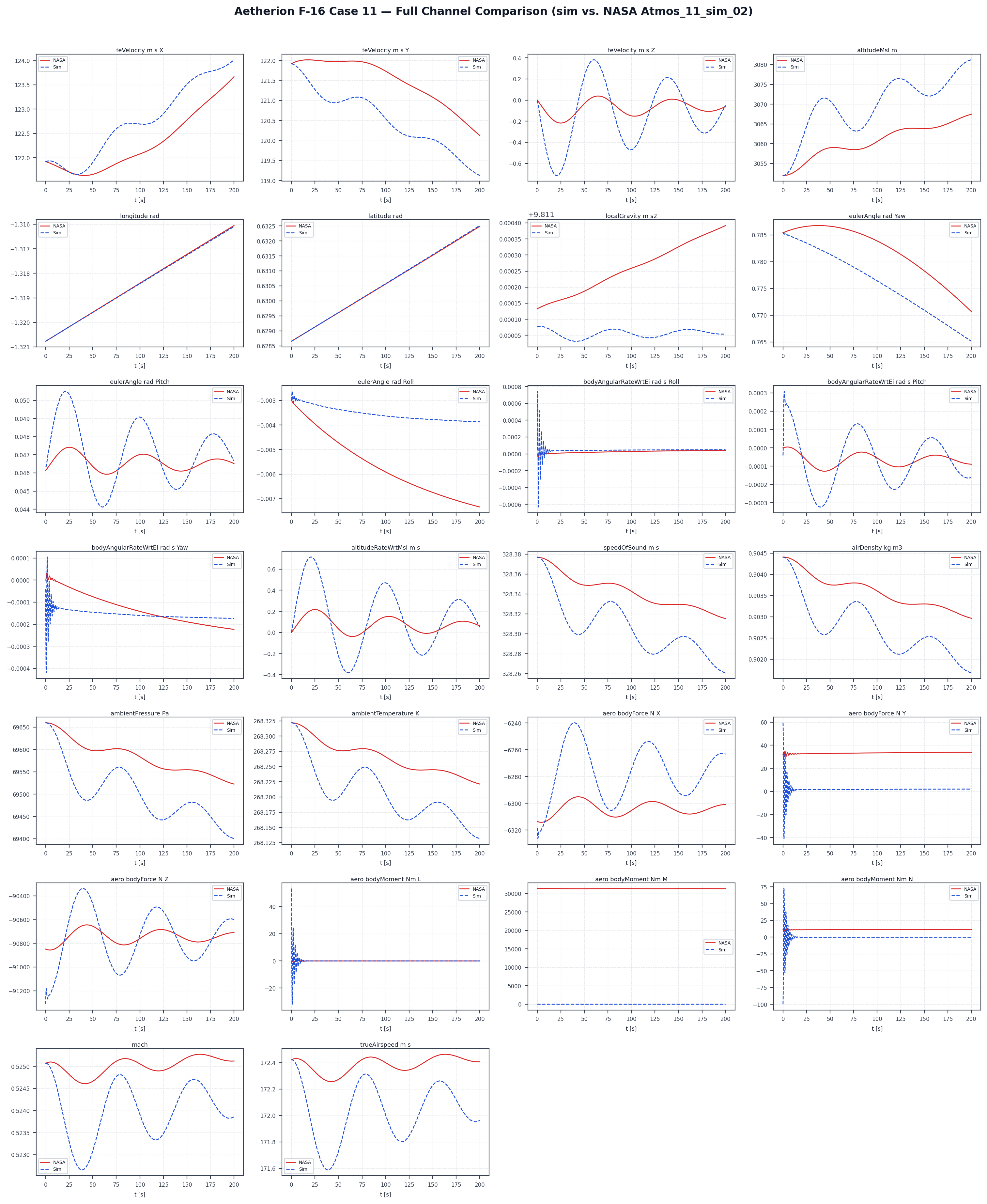
Scenario 11 simulation overview. Aetherion (blue dashed) vs NASA Atmos_11_sim_05 (red).
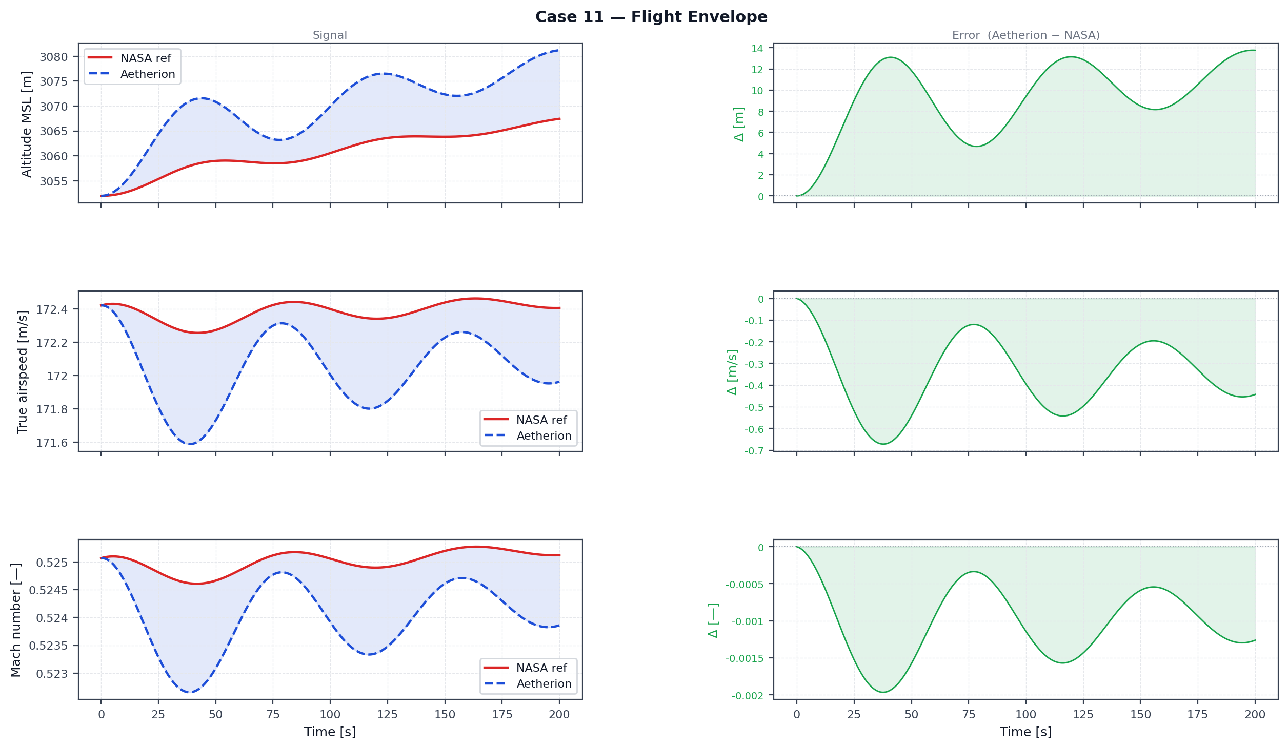
Scenario 11 flight envelope — altitude, TAS, Mach. Aetherion (blue dashed) vs NASA Atmos_11_sim_05 (red).
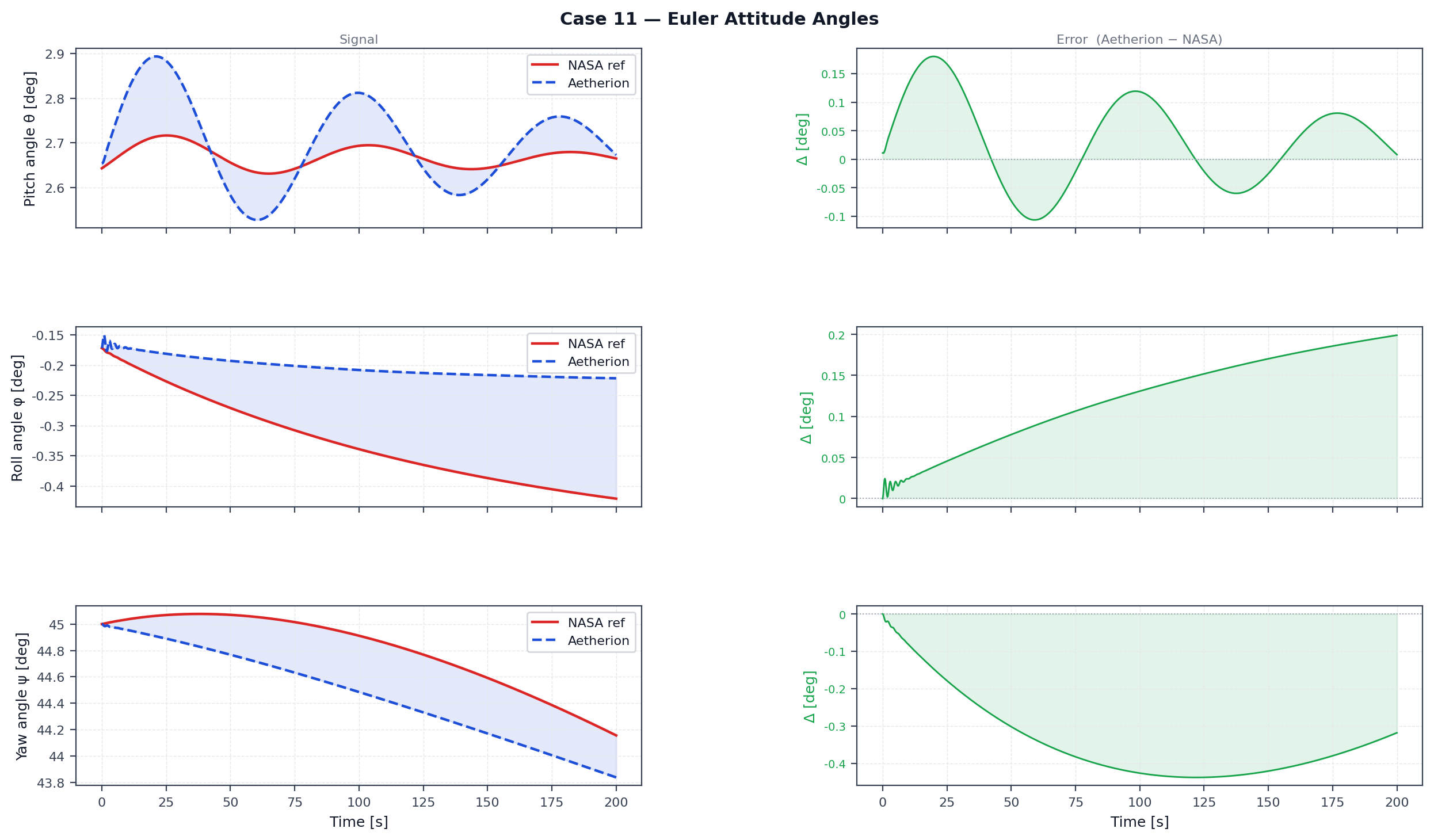
Scenario 11 Euler attitude angles — pitch, roll, yaw. Aetherion (blue dashed) vs NASA Atmos_11_sim_05 (red).
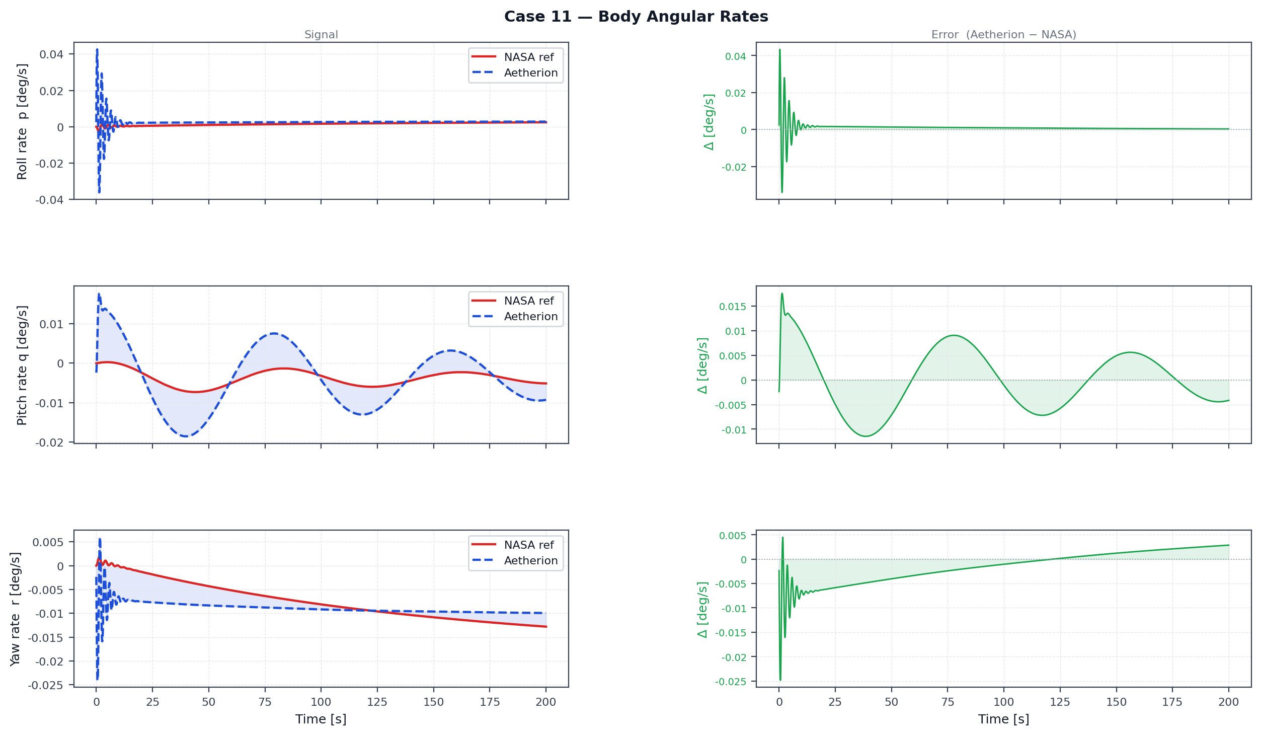
Scenario 11 body angular rates — roll, pitch, yaw rates. Aetherion (blue dashed) vs NASA Atmos_11_sim_05 (red).
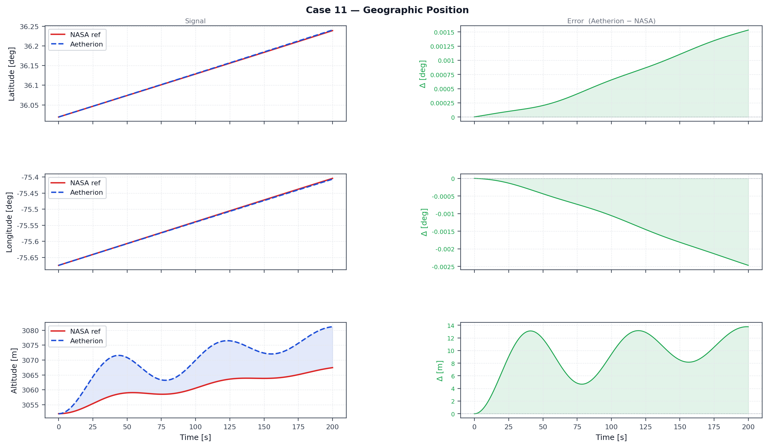
Scenario 11 geodetic position — altitude, latitude, longitude. Aetherion (blue dashed) vs NASA Atmos_11_sim_05 (red).
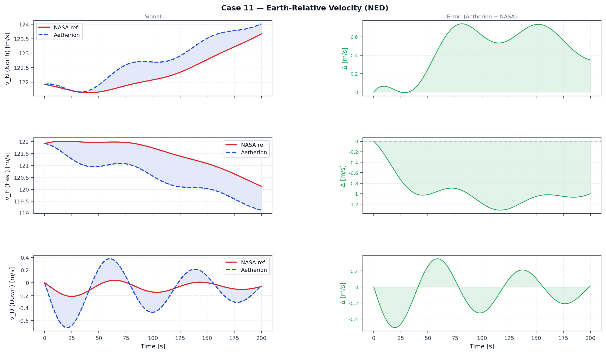
Scenario 11 NED velocity components — North, East, Down. Aetherion (blue dashed) vs NASA Atmos_11_sim_05 (red).
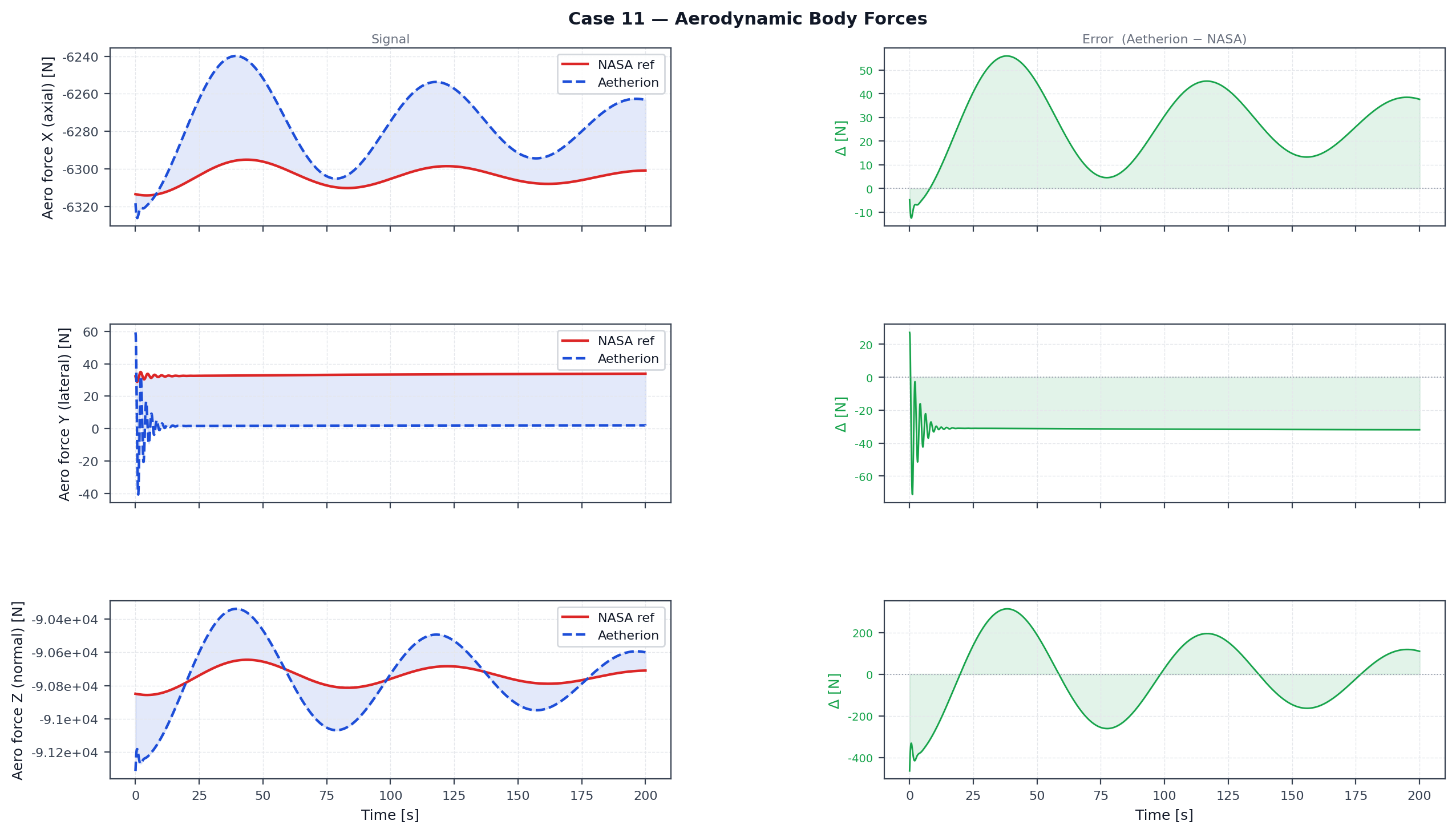
Scenario 11 aerodynamic body forces — X, Y, Z. Aetherion (blue dashed) vs NASA Atmos_11_sim_05 (red).
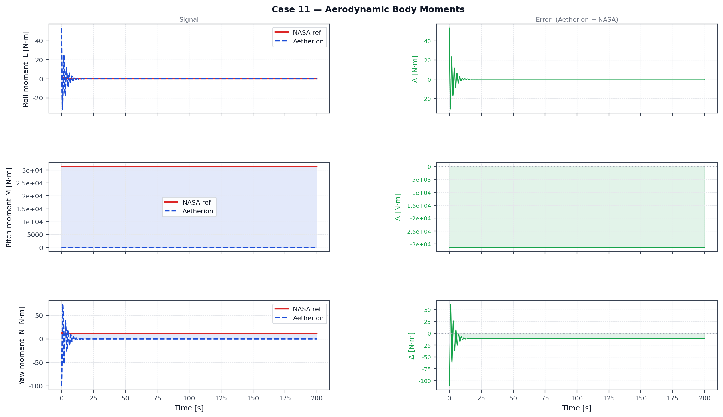
Scenario 11 aerodynamic body moments — L, M, N. Aetherion (blue dashed) vs NASA Atmos_11_sim_05 (red).
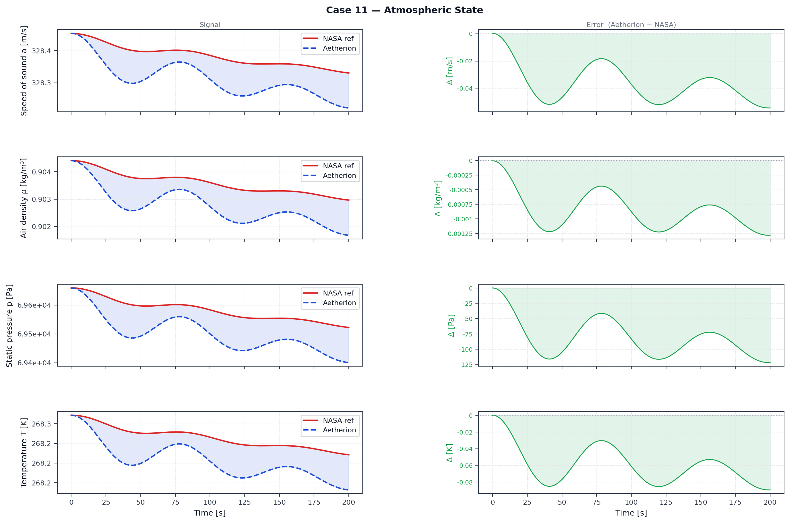
Scenario 11 atmosphere — temperature, density, pressure. Aetherion (blue dashed) vs NASA Atmos_11_sim_05 (red).
F-16 Supersonic Trim Check (NASA TM-2015-218675 Atmospheric Check-Case 12)
Scenario Overview
Check-Case 12 is the supersonic analogue of Check-Case 11. The same F-16 vehicle flies steady straight-and-level flight, but at Mach ≈ 2.01 and 30 013 ft altitude instead of the subsonic condition. As in Case 11, the simulation is open-loop: control surfaces and throttle are held fixed at the trim values for the entire 200 s run; no autopilot or SAS is active.
Key aerodynamic differences from Case 11:
At supersonic speed, wave drag dominates. The required throttle rises from 13.9 % (subsonic) to 56.9 % to overcome the much higher drag.
The trim angle of attack is −0.742° (slightly nose-down) rather than +2.639° (nose-up), because supersonic lift is generated more efficiently at a lower α.
The trim elevator deflection is −1.528° (smaller than the subsonic −3.233°) due to the different moment balance at Mach 2.
The rotating-Earth relief is three times larger than in Case 11 — 1.34 % of the weight, 275 lbf — because both the Eötvös and the path-curvature terms grow with speed. See Trimming over a rotating, curved Earth.
The reused class is F16SteadyFlightSimulator; the only differences from
Case 11 are the flight-condition constants compiled into
F16SupersonicTrim.cpp.
Initial and Flight Conditions
Parameter |
Value |
|---|---|
Location |
36.019° N, 75.674° W (Kitty Hawk, NC) |
Altitude |
30 013 ft (9 147.96 m) |
Heading |
45° NE |
TAS (initial) |
≈ 2 000 ft/s (1 184.96 KTAS) |
vN = vE |
1 414.2 ft/s = 430.9 m/s |
vD |
0 ft/s |
Body rates |
all zero (trim) |
Simulation duration |
200 s |
Trim Result
Quantity |
Aetherion |
NASA ref |
|---|---|---|
Mach (trim) |
2.0104 |
2.01045 |
α (trim) |
−0.7415° |
−0.7416° (sims 04 and 05; sim 02: −0.7366°) |
δe (trim) |
−1.528° |
n/a (not tabulated in CSV) |
Throttle (trim) |
56.89 % |
n/a |
Thrust (trim) |
54 083 N (12 158 lbf) |
n/a |
Speed of sound |
303.11 m/s (994.44 ft/s) |
994.79 ft/s |
The trim solution agrees with NASA simulations 04 and 05 within 0.0001°.
Step-Size Convergence
Unlike the closed-loop scenarios (13.1–13.4), the supersonic trim is an open-loop problem with no stiff controller gains. The Radau IIA implicit integrator converges to the same trajectory for all tested step sizes:
dt [s] |
alt @ 200 s [ft] |
Δalt [ft] |
Mach |
pitch [°] |
|---|---|---|---|---|
0.10 |
30 012.3 |
−0.7 ✓ |
2.010434 |
−0.742 |
0.05 |
30 012.3 |
−0.7 ✓ |
2.010434 |
−0.742 |
0.02 |
30 012.3 |
−0.7 ✓ |
2.010434 |
−0.742 |
dt = 0.1 s is recommended for Case 12 (10× faster than the closed-loop cases, no accuracy penalty).
Recommended Run Command
F16SupersonicTrim --endTime 200 --timeStep 0.1 \
                  --outputFileName f16_s12_sim.csv
The reference CSVs Atmos_12_sim_02/04/05.csv and the plot script
plot_f16_s12_nasa.py are copied to the build directory post-build.
Validation Results at t = 200 s
Quantity |
Aetherion |
NASA sim 02 |
|---|---|---|
Altitude |
30 012.3 ft (9 147.8 m) |
30 256.9 ft (9 222.1 m) |
Δ altitude |
−0.7 ft |
+243.9 ft |
TAS |
609.59 m/s (1 185.0 KTAS) |
610.28 m/s (1 186.3 KTAS) |
Mach |
2.010434 |
2.014849 |
Pitch θ |
−0.742° |
−0.616° |
Roll φ |
−0.177° |
−0.559° |
Yaw ψ |
46.248° |
45.657° |
Note
Simulation 02 is the only NASA reference that runs to 200 s, and it is not in trim: it climbs 244 ft, peaking 459 ft high on the way. Aetherion holds the trim altitude to 0.7 ft over the same 200 s, as NASA simulations 04 and 05 do over their 180 s (0.9 ft and 0.1 ft). Up to release 0.14.1 Aetherion climbed 505 ft here; see Trimming over a rotating, curved Earth. Against simulation 05 at t = 180 s: yaw 46.143° vs 46.172°, roll −0.165° vs −0.149°, pitch −0.7417° vs −0.7417°. The figures below plot against simulation 05.
Validation Figures
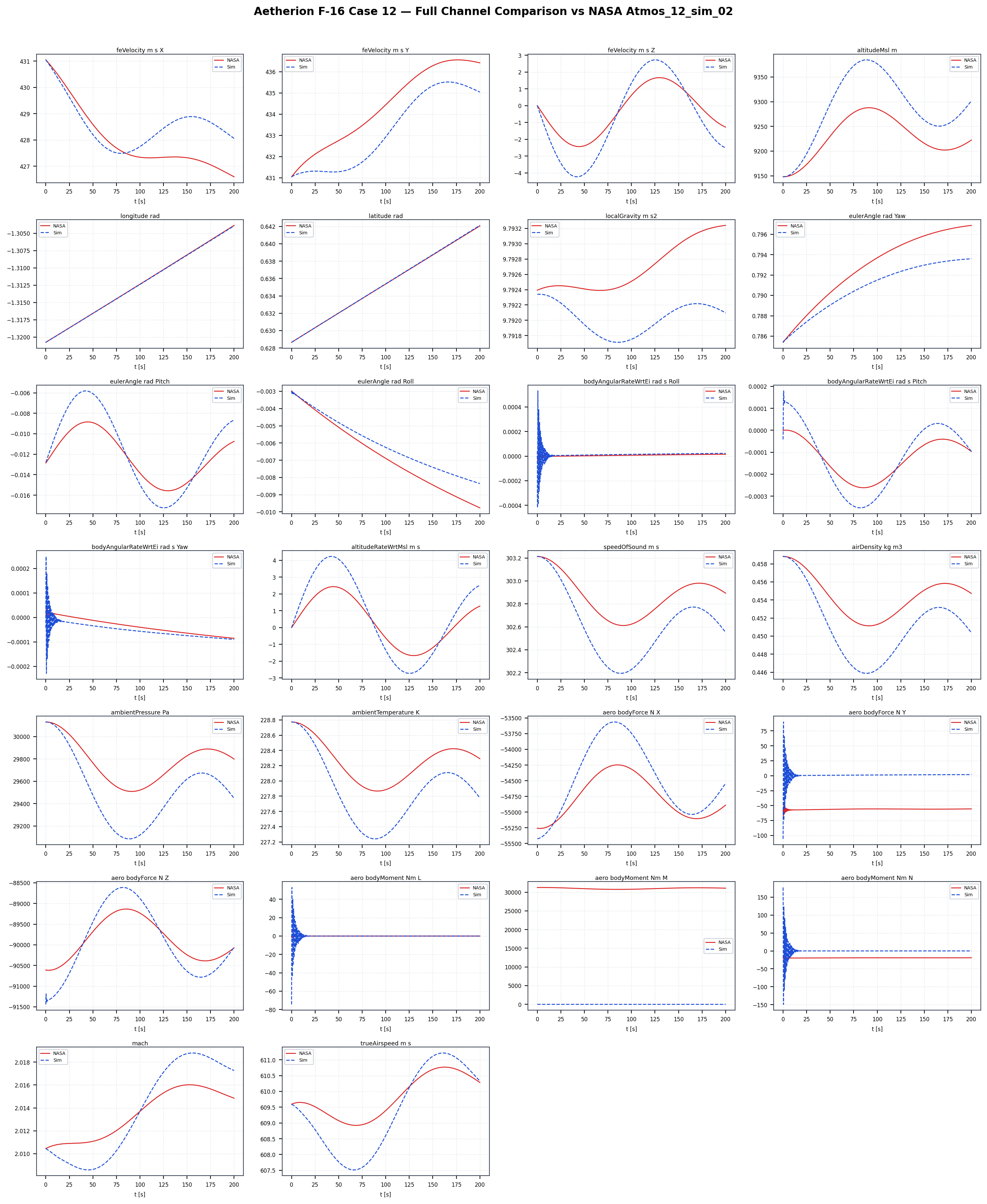
Case 12 simulation overview. Aetherion (blue dashed) vs NASA Atmos_12_sim_05 (red).
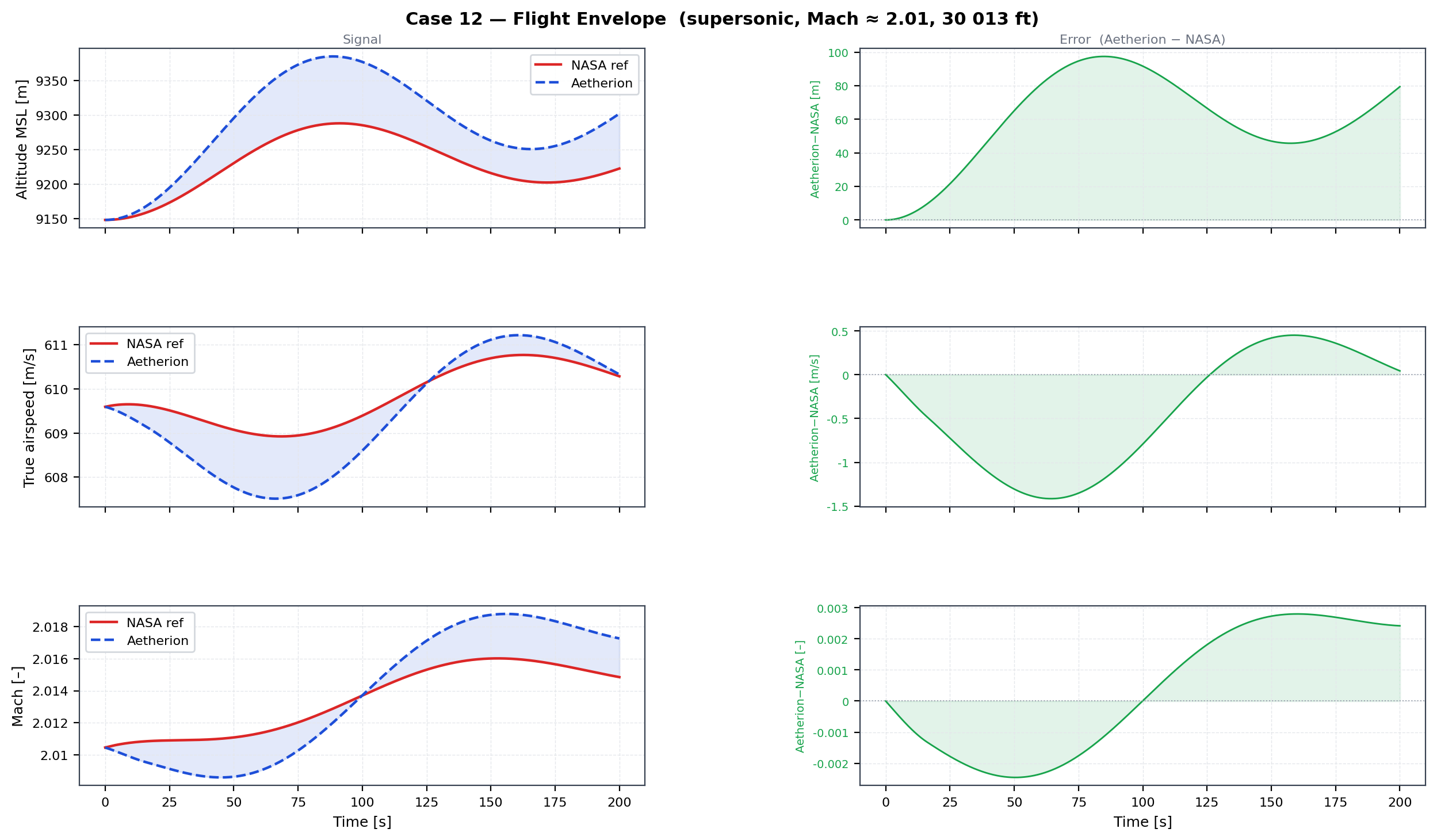
Case 12 flight envelope — altitude, TAS, Mach. Aetherion (blue dashed) vs NASA Atmos_12_sim_05 (red).
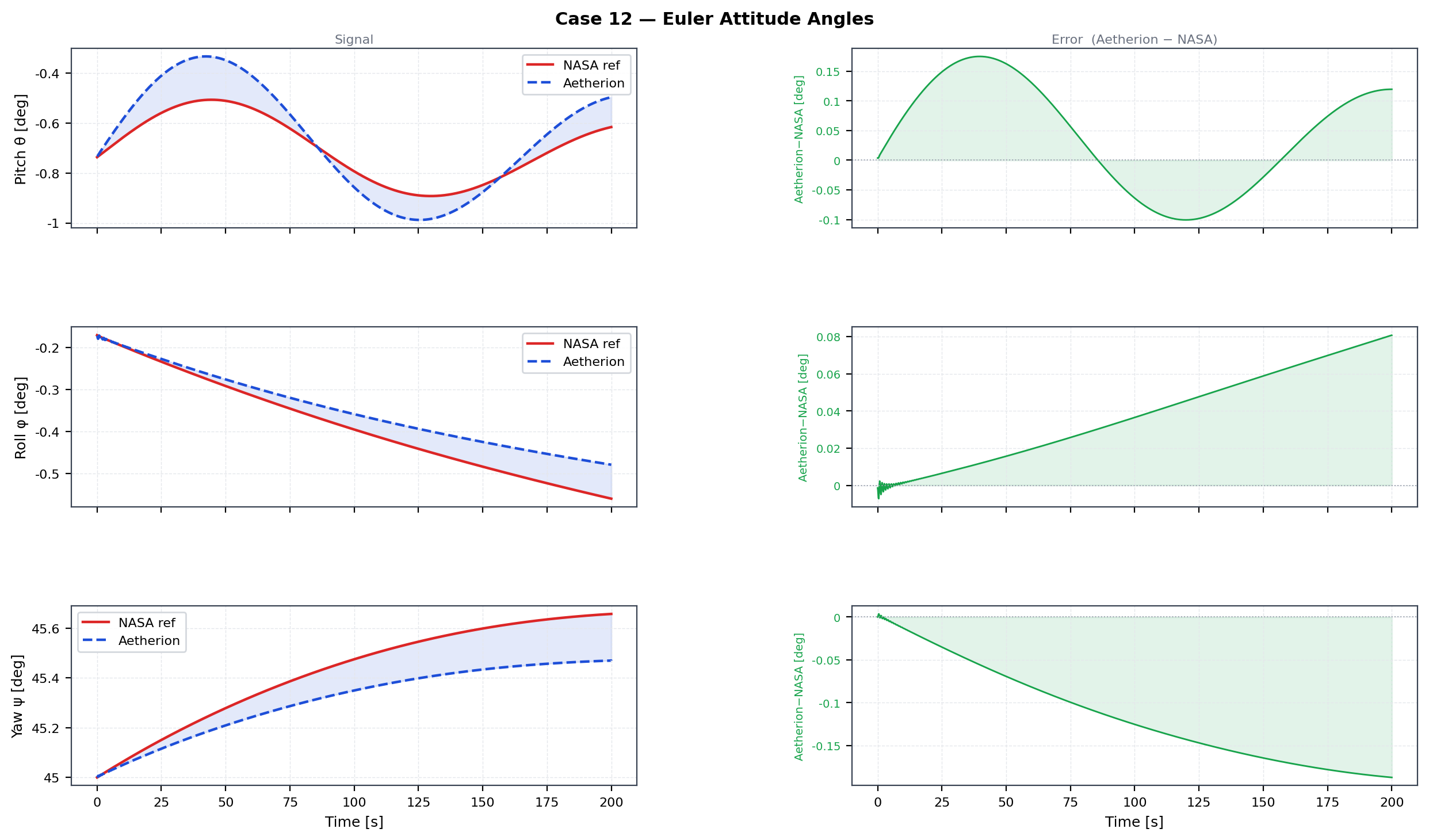
Case 12 Euler attitude angles — pitch, roll, yaw. Aetherion (blue dashed) vs NASA Atmos_12_sim_05 (red).
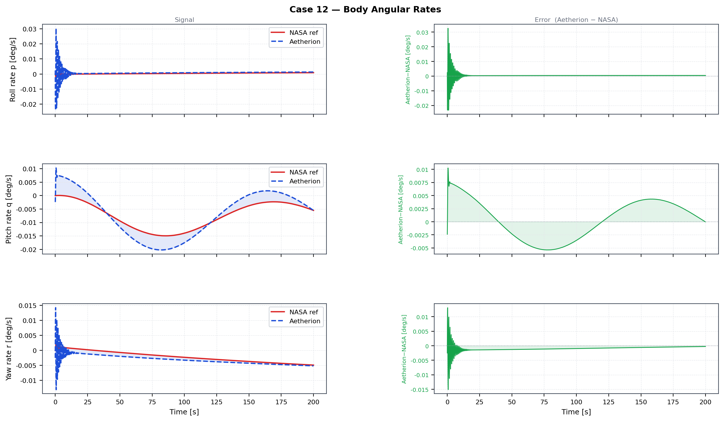
Case 12 body angular rates — roll, pitch, yaw rates. Aetherion (blue dashed) vs NASA Atmos_12_sim_05 (red).
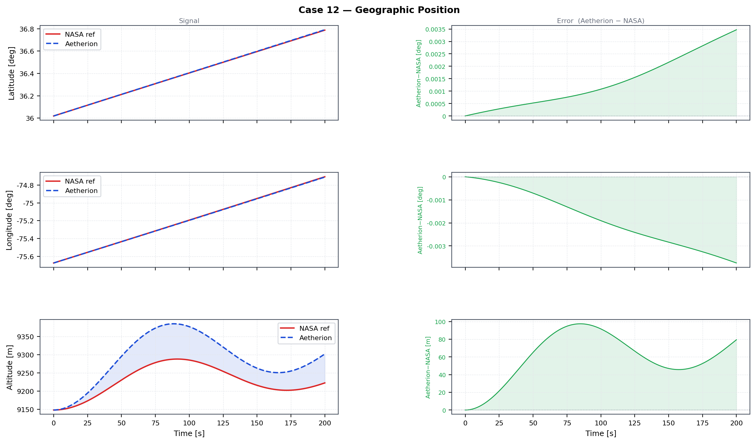
Case 12 geodetic position — altitude, latitude, longitude. Aetherion (blue dashed) vs NASA Atmos_12_sim_05 (red).
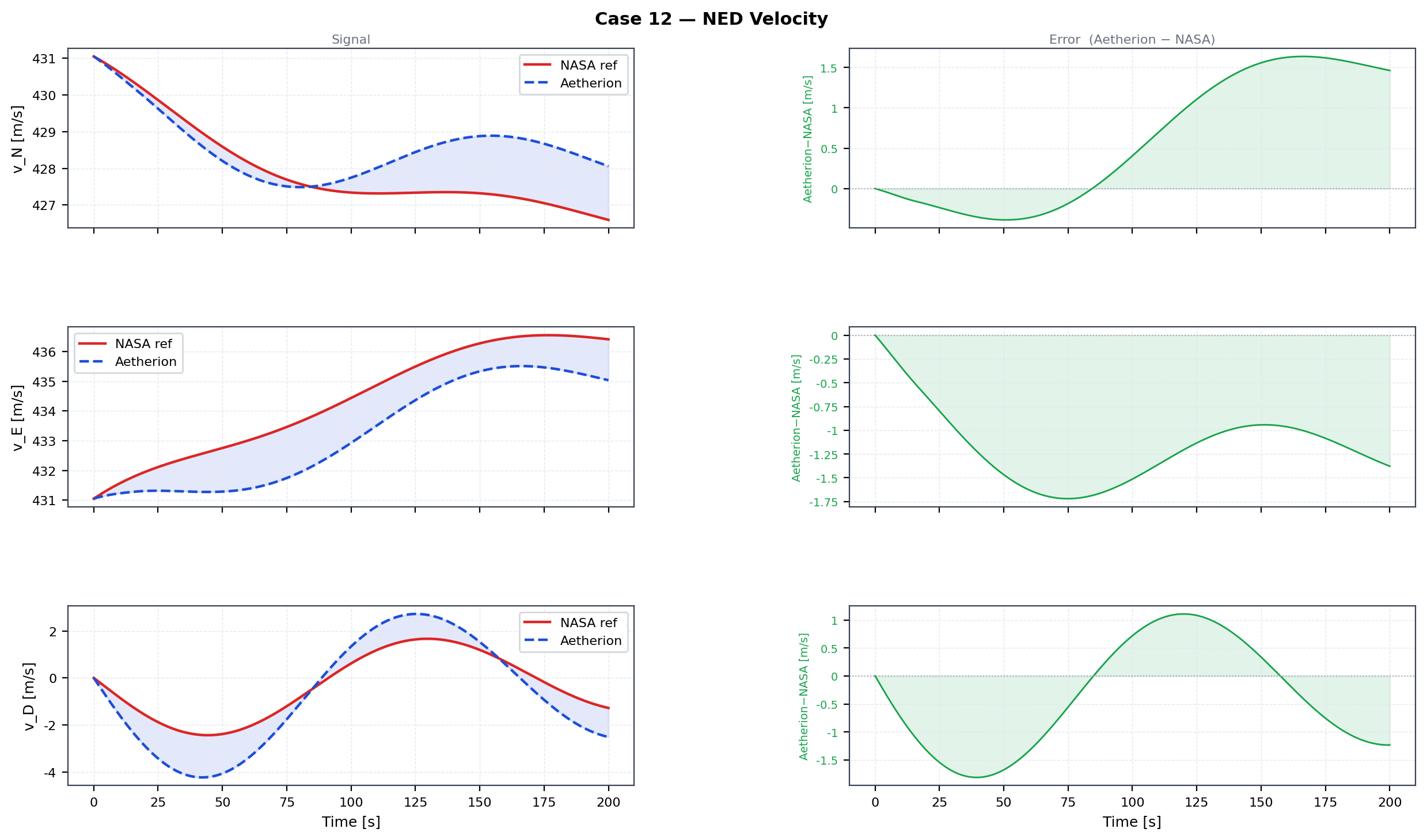
Case 12 NED velocity components — North, East, Down. Aetherion (blue dashed) vs NASA Atmos_12_sim_05 (red).
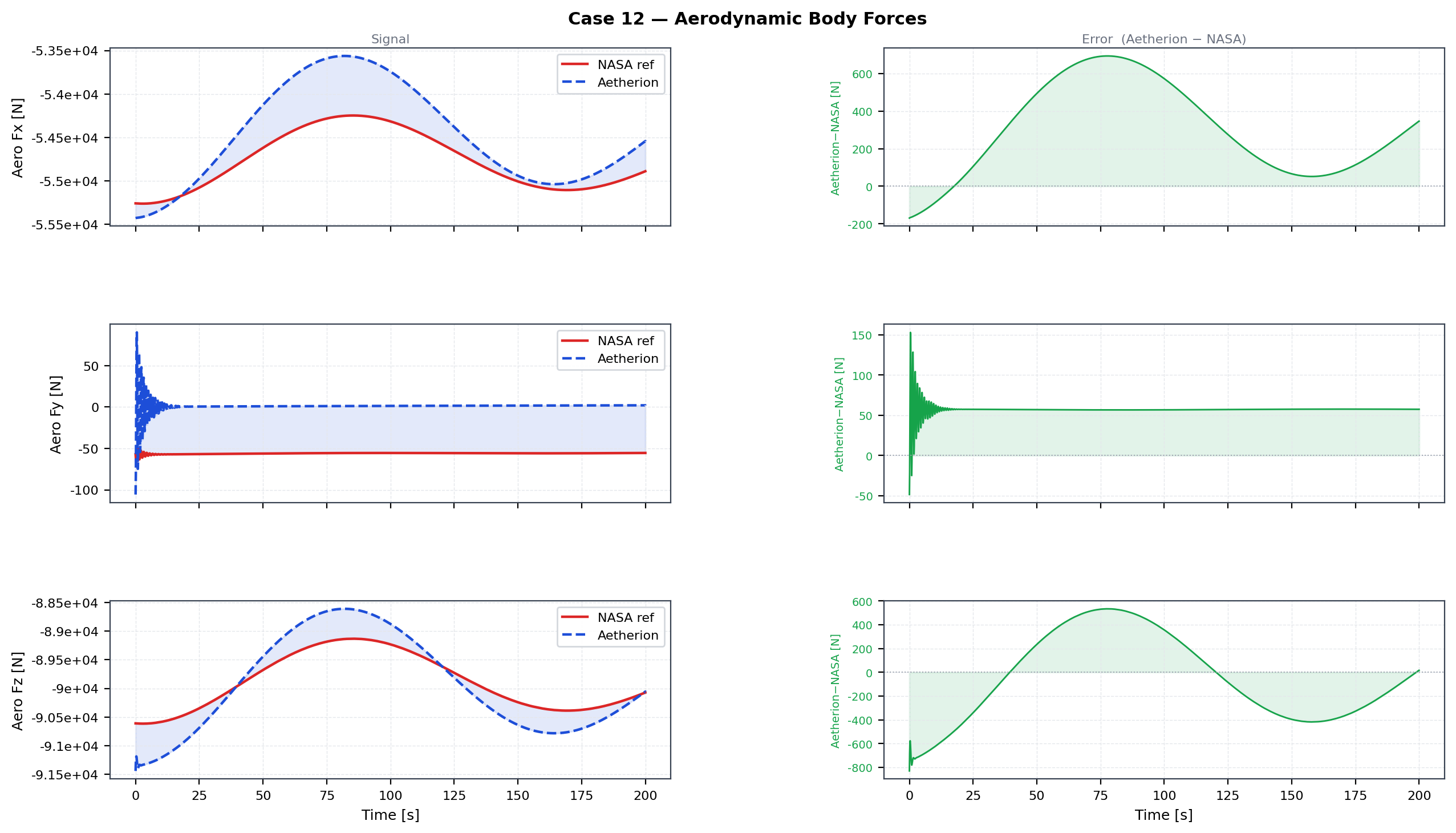
Case 12 aerodynamic body forces — X, Y, Z. Aetherion (blue dashed) vs NASA Atmos_12_sim_05 (red).
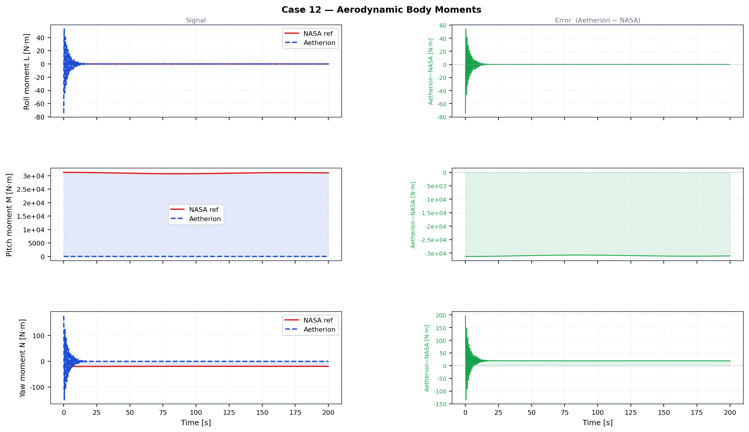
Case 12 aerodynamic body moments — L, M, N. Aetherion (blue dashed) vs NASA Atmos_12_sim_05 (red).
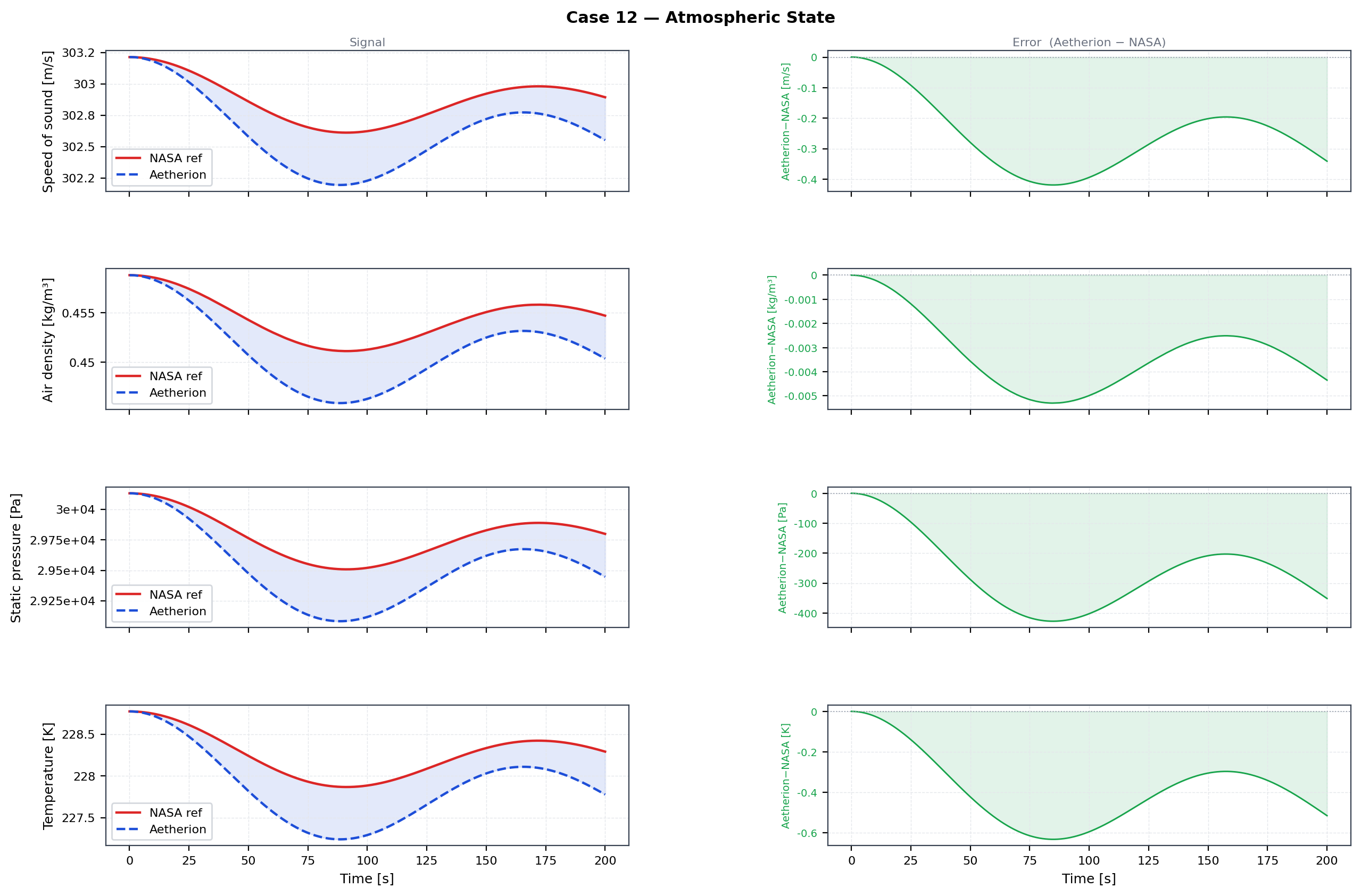
Case 12 atmosphere — temperature, density, pressure. Aetherion (blue dashed) vs NASA Atmos_12_sim_05 (red).
F-16 Subsonic Altitude Change (NASA TM-2015-218675 Atmospheric Scenario 13.1)
Scenario overview
Starting from the same Kitty Hawk trim as Scenario 11, the F-16 executes
a closed-loop +100 ft altitude change driven by the NASA LQR stability-
augmentation system (SAS) and altitude-hold autopilot defined in
F16_control.dml.
The control architecture is:
Inner loop — Linear Quadratic Regulator (LQR) with 4-state longitudinal (V, α, q, θ) and 4-state lateral-directional (φ, β, p, r) gain matrices.
Outer loop — altitude-error-to-pitch-command compensator (Kalt = −0.05 °/ft), airspeed hold via throttle, and heading hold via bank angle command.
All LQR gains and trim values are read at runtime from
data/F16_S119_source/F16_control.dml; no gains are hardcoded.
Initial and command conditions
Parameter |
Value |
|---|---|
Location |
36.019° N, 75.674° W (Kitty Hawk, NC) |
Altitude (initial) |
10 013 ft (3 051.96 m) |
Altitude command (altCmd) |
10 113 ft (+100 ft step, applied at t = 5 s) |
Heading |
45° NE |
TAS (trim) |
335.15 KTAS (172.4 m/s) |
Mach (trim) |
0.525 |
KEAS command |
computed from US1976 atmosphere at trim altitude |
Simulation duration |
20 s |
Numerical step-size requirement
The closed-loop LQR plant is stiff — the high gains create fast eigenvalues that exceed the Radau IIA stability boundary at dt = 0.1 s. A convergence study confirms:
dt [s] |
alt @ 20 s [ft] |
Δ vs command [ft] |
pitch [°] |
roll [°] |
|---|---|---|---|---|
0.10 |
10 085.7 |
−27.3 ❌ |
3.77 |
−4.08 |
0.05 |
10 109.1 |
−3.9 |
2.83 |
−2.16 |
0.02 |
10 113.1 |
+0.1 ✓ |
2.65 |
−0.10 |
0.01 |
10 113.1 |
+0.1 ✓ |
2.65 |
−0.10 |
Use --timeStep 0.02 (or smaller) for accurate closed-loop results.
Recommended run command
F16AltitudeChange --endTime 20 --timeStep 0.02 \
                  --outputFileName f16_s13p1.csv
The reference CSVs Atmos_13p1_sim_02/04/05.csv and the plot script
plot_f16_s13p1_nasa.py are copied to the build directory post-build.
Controller architecture
The GNC model (F16_control.dml) implements a two-loop architecture.
All gains and trim values are read at runtime from the DML file.
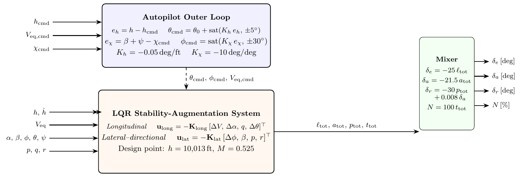
F-16 GNC two-loop control architecture: autopilot outer loop (altitude, airspeed and heading hold) feeding commanded states to the LQR stability-augmentation inner loop.
- Inputs:
sensor feedbacks (\(h\), \(V_\mathrm{eq}\), \(\alpha\), \(\beta\), \(\phi\), \(\theta\), \(\psi\), \(p\), \(q\), \(r\)), autopilot commands (\(h_\mathrm{cmd}\), \(V_\mathrm{eq,cmd}\), \(\chi_\mathrm{cmd}\), lateral offset), trim feed-forwards (\(\ell_\mathrm{trim}\), \(t_\mathrm{trim}\)), mode flags (
sasOn,apOn).- Outputs:
\(\delta_e\) [deg, TED+], \(\delta_a\) [deg, LWD+], \(\delta_r\) [deg, TEL+], \(N\) [0–100 %].
LQR inner loop — longitudinal channel
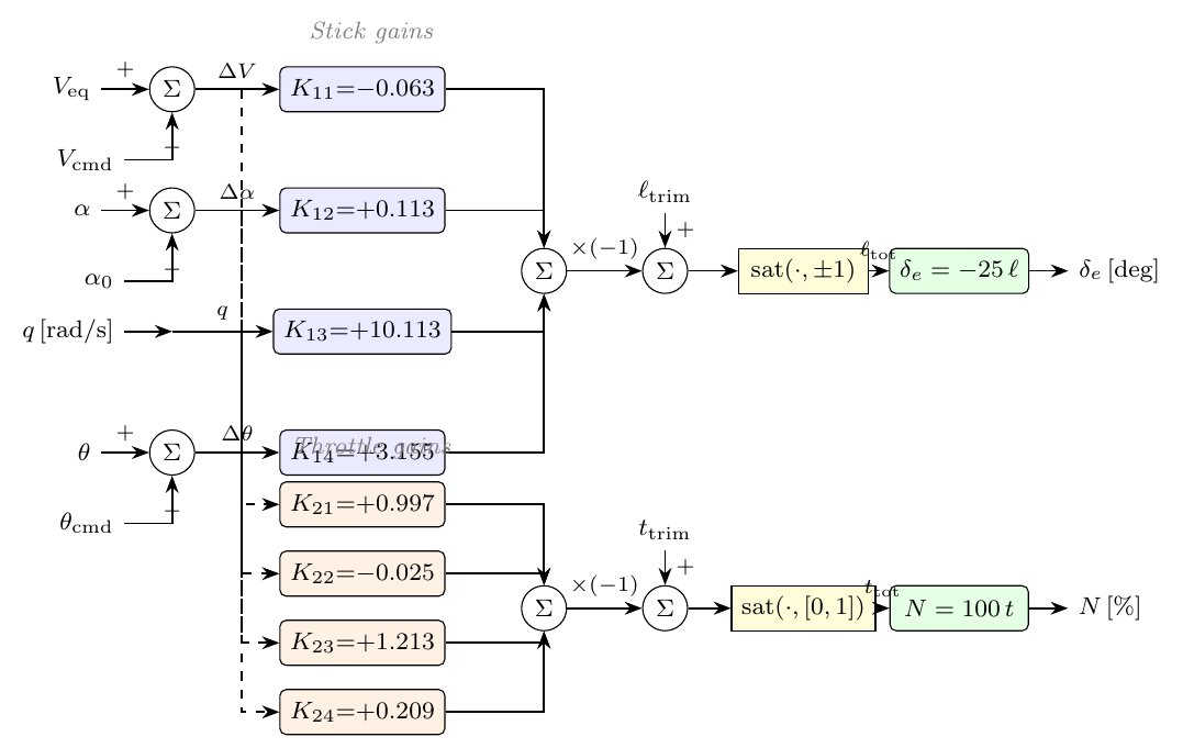
Longitudinal LQR signal-flow: four state errors (\(\Delta V\), \(\Delta\alpha\), \(q\), \(\Delta\theta\)) multiplied by gain matrices \(\mathbf{K}_\mathrm{long}\) and \(\mathbf{K}_\mathrm{throt}\), summed, negated, added to the trim feed-forward, saturated, and scaled to elevator \(\delta_e\) and throttle \(N\). Dashed lines indicate the throttle channel reuses the same state errors.
LQR inner loop — lateral-directional channel
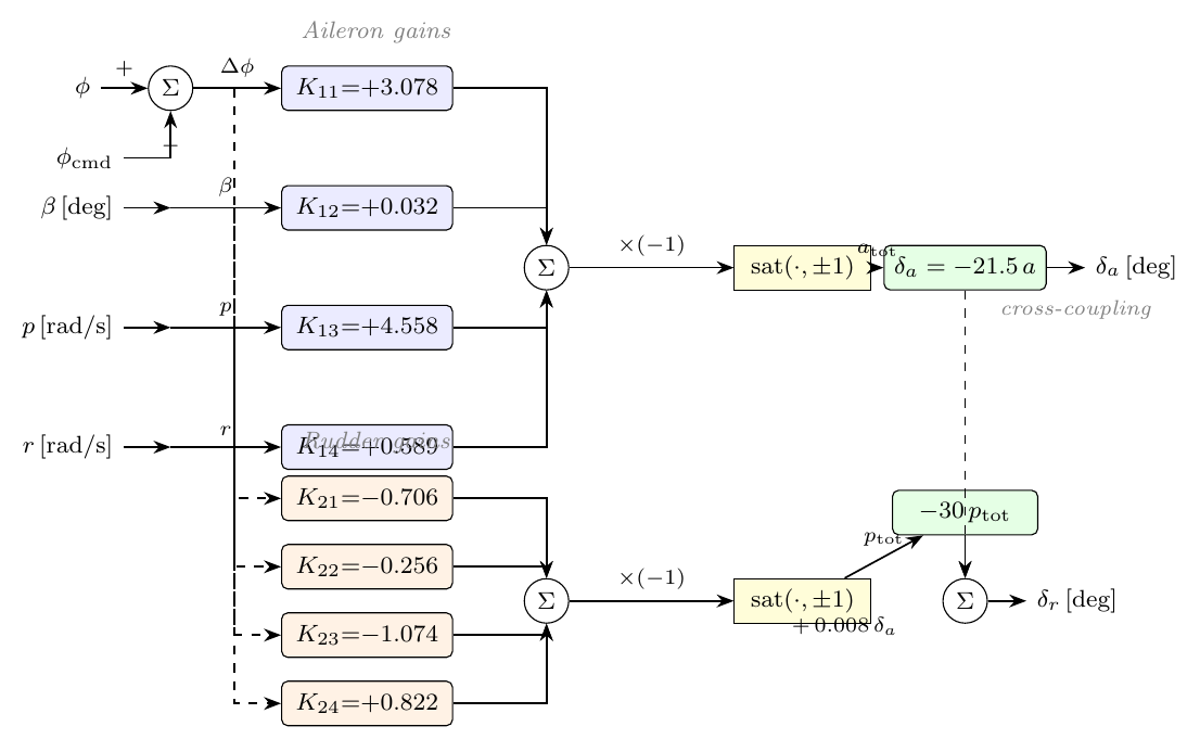
Lateral-directional LQR signal-flow: four state errors (\(\Delta\phi\), \(\beta\), \(p\), \(r\)) multiplied by gain matrices \(\mathbf{K}_\mathrm{ail}\) and \(\mathbf{K}_\mathrm{rdr}\), summed and negated to aileron \(\delta_a\) and rudder \(\delta_r\). The aileron-to-rudder cross-coupling \(\delta_r \mathrel{+}= 0.008\,\delta_a\) is shown by the dashed feedback path.
Trim result (Scenario 13.1)
Identical to Scenario 11 (same initial conditions):
Quantity |
Aetherion |
NASA ref |
|---|---|---|
α (trim) |
2.6391° |
2.6389° (sim 05; sim 02: 2.6433°, not in trim) |
δe (trim) |
−3.233° |
−3.24° |
Throttle (trim) |
13.87 % |
13.90 % |
Validation results at t = 20 s (dt = 0.02 s)
Quantity |
Aetherion |
NASA sim 05 |
|---|---|---|
Altitude |
10 112.9 ft (3 082.4 m) |
10 112.6 ft (3 082.3 m) |
Δ altitude (change from t=0) |
+99.9 ft |
+99.6 ft |
TAS |
172.69 m/s |
172.69 m/s |
Mach |
0.5261 |
0.5261 |
Pitch θ |
2.660° |
2.660° |
Roll φ |
−0.10° |
−0.10° |
Peak errors against simulation 05 over the 20 s: altitude ±0.11 m, pitch ±0.63°, roll ±0.004°. The pitch peak is confined to the first half second after the step, where the two zero-order-hold controllers sample the command at different instants. The final state (t = 20 s) agrees to within 0.3 ft altitude and 0.001° in both pitch and roll.
Validation figures
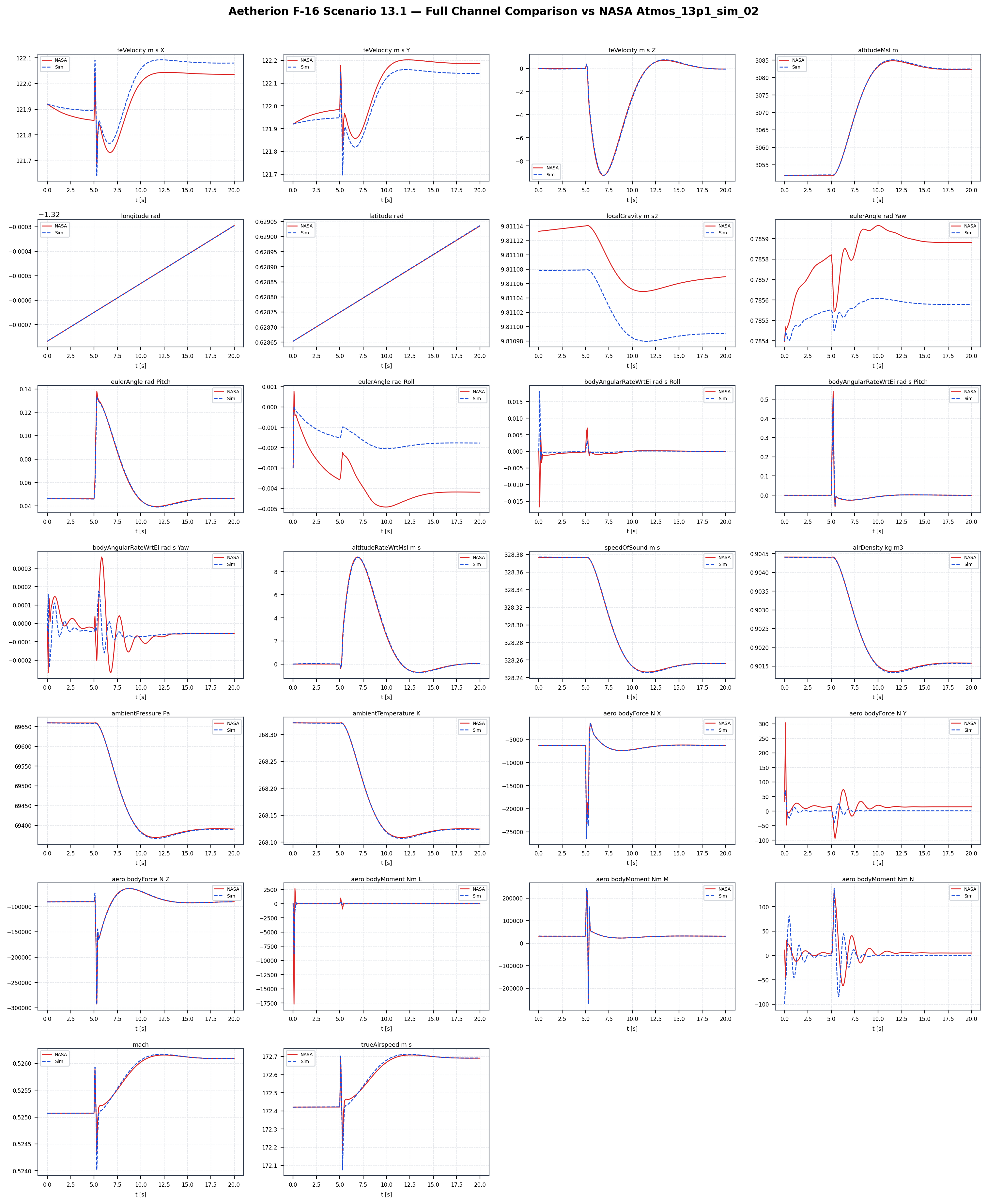
Scenario 13.1 simulation overview. Aetherion (blue dashed) vs NASA Atmos_13p1_sim_05 (red).
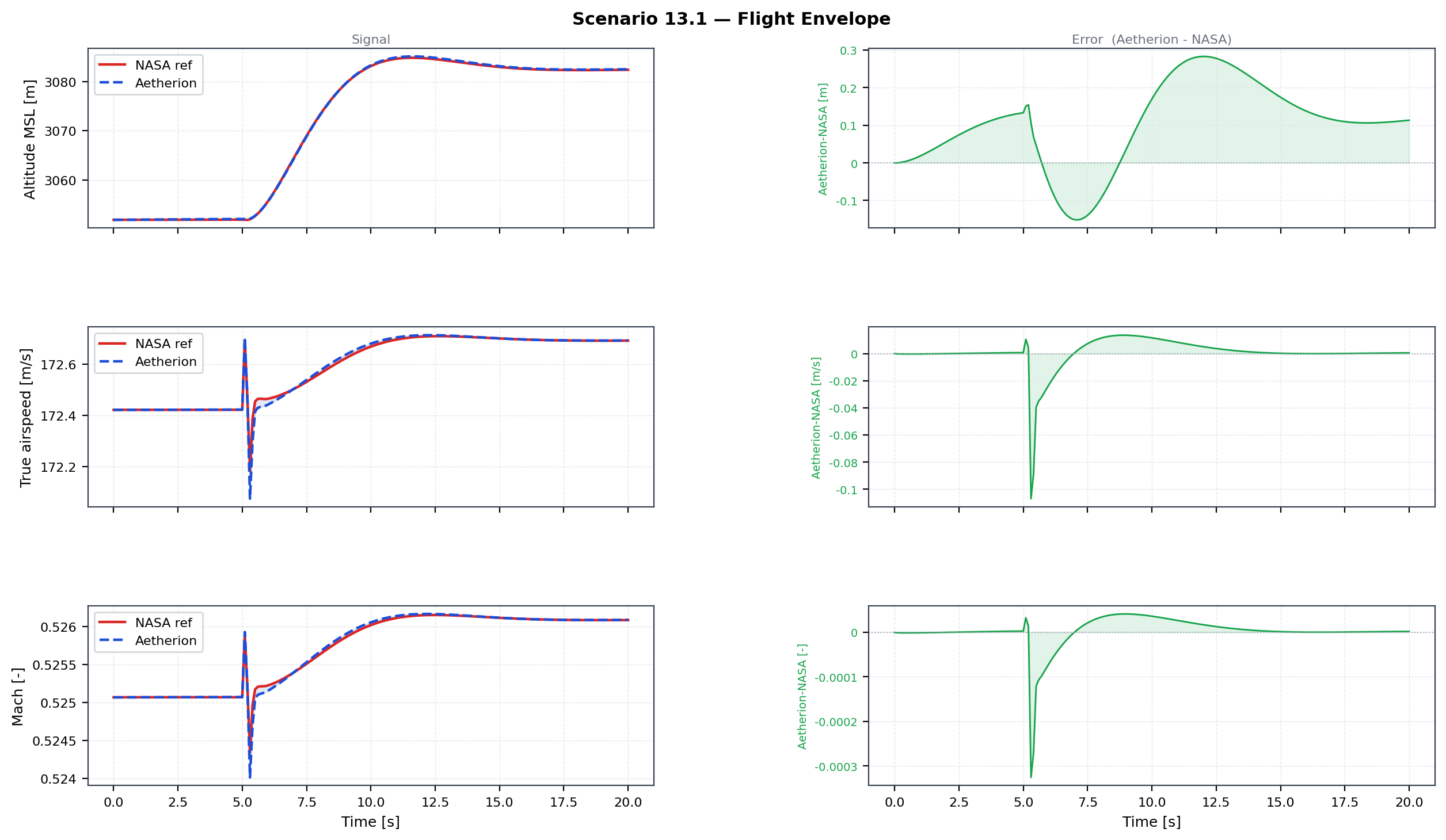
Scenario 13.1 flight envelope — altitude, TAS, Mach. Aetherion (blue dashed) vs NASA Atmos_13p1_sim_05 (red).
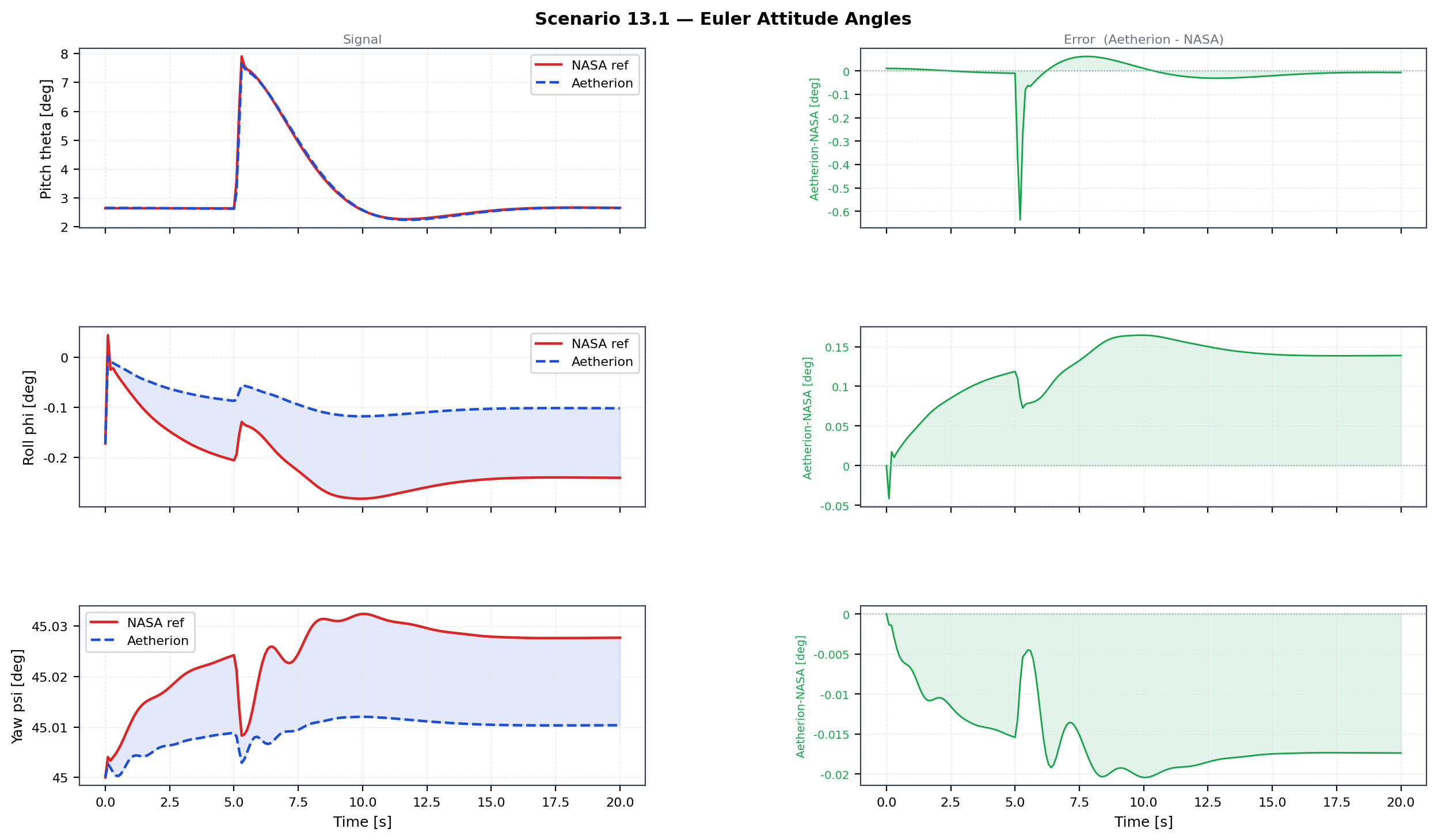
Scenario 13.1 Euler attitude angles — pitch, roll, yaw. Aetherion (blue dashed) vs NASA Atmos_13p1_sim_05 (red).
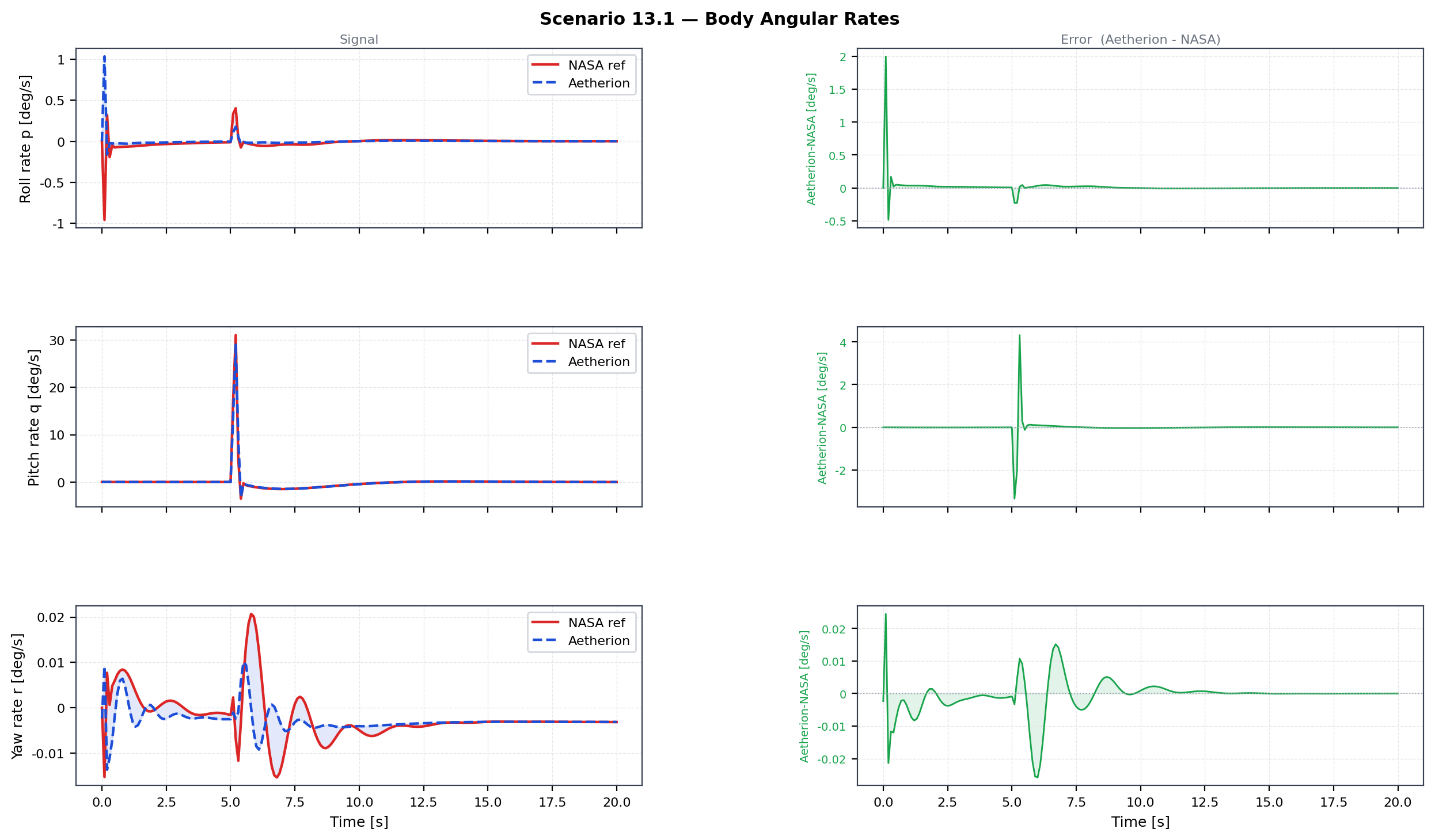
Scenario 13.1 body angular rates — roll, pitch, yaw rates. Aetherion (blue dashed) vs NASA Atmos_13p1_sim_05 (red).
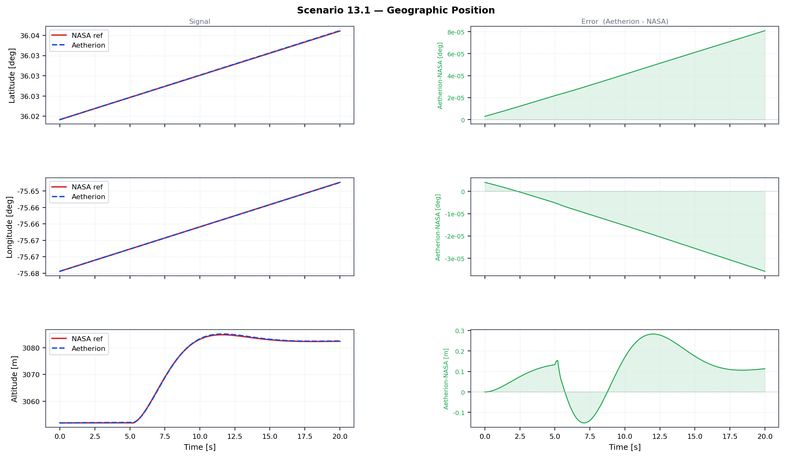
Scenario 13.1 geodetic position — altitude, latitude, longitude. Aetherion (blue dashed) vs NASA Atmos_13p1_sim_05 (red).
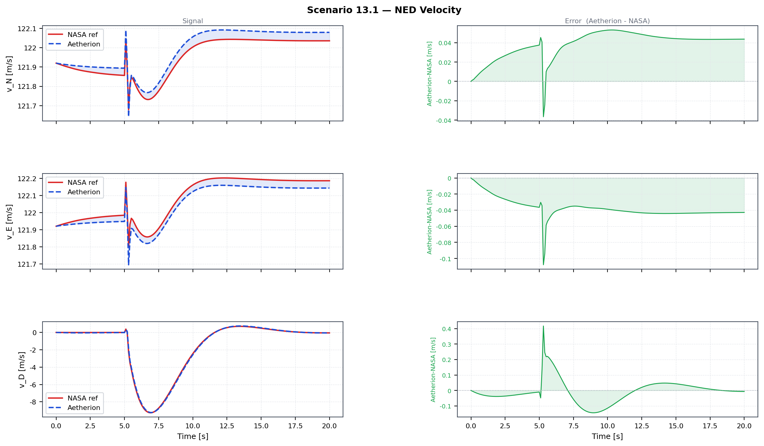
Scenario 13.1 NED velocity components — North, East, Down. Aetherion (blue dashed) vs NASA Atmos_13p1_sim_05 (red).
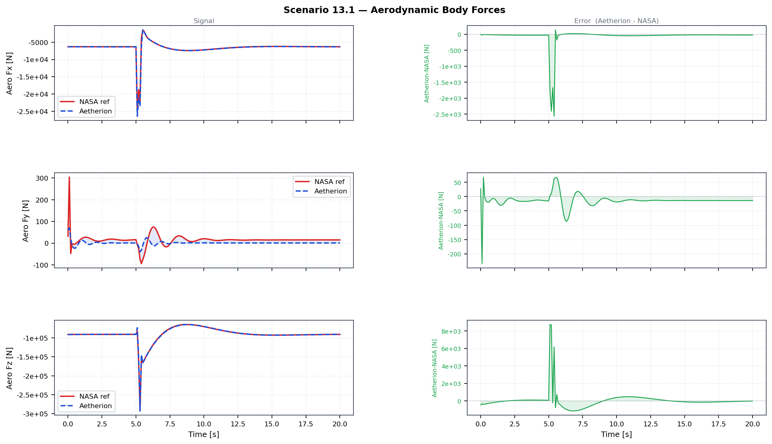
Scenario 13.1 aerodynamic body forces — X, Y, Z. Aetherion (blue dashed) vs NASA Atmos_13p1_sim_05 (red).
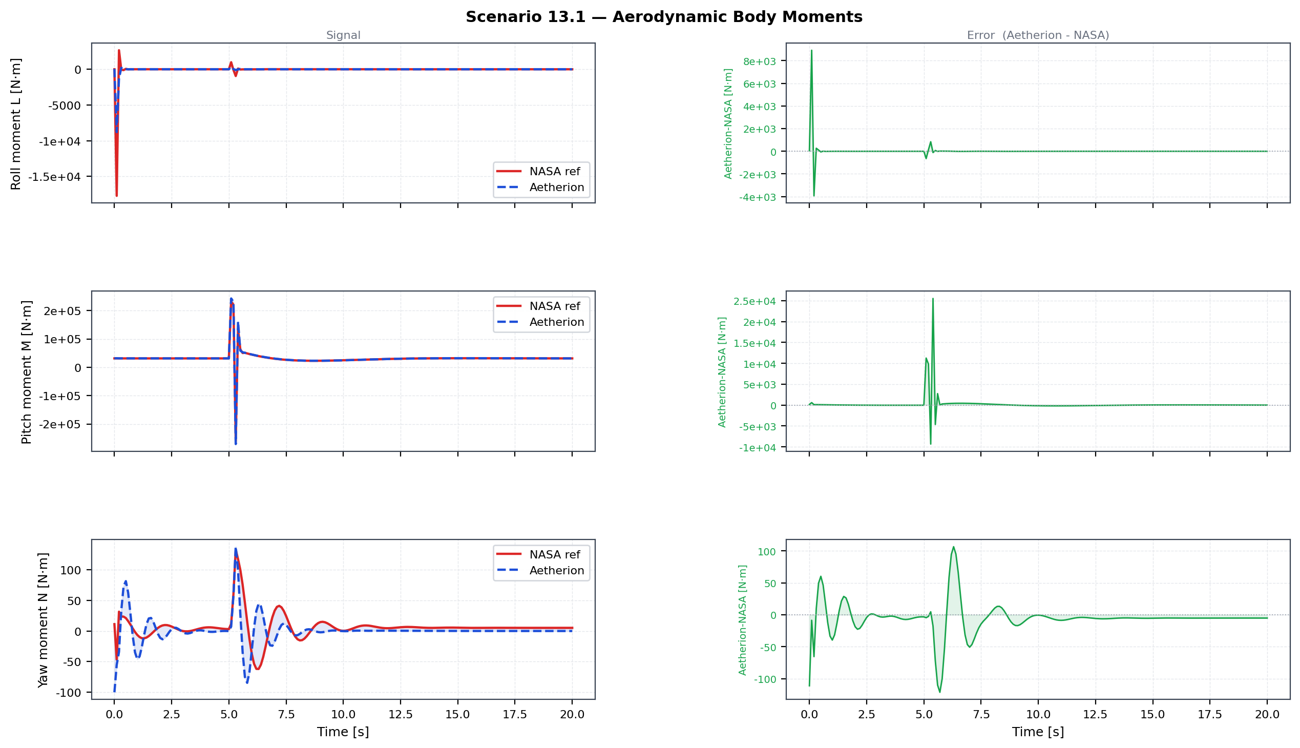
Scenario 13.1 aerodynamic body moments — L, M, N. Aetherion (blue dashed) vs NASA Atmos_13p1_sim_05 (red).
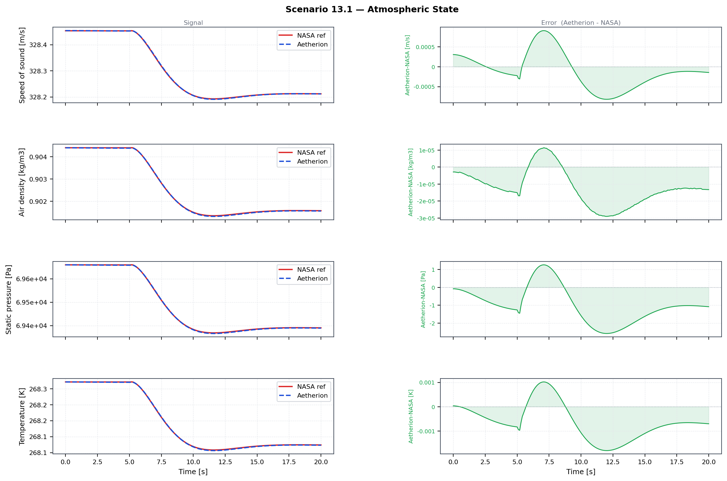
Scenario 13.1 atmosphere — temperature, density, pressure. Aetherion (blue dashed) vs NASA Atmos_13p1_sim_05 (red).
F-16 Subsonic Airspeed Change (NASA TM-2015-218675 Atmospheric Scenario 13.2)
Scenario overview
Starting from the same Kitty Hawk trim as Scenario 11, the F-16 executes
a closed-loop −10 kt KEAS airspeed reduction driven by the NASA LQR SAS
and throttle-hold autopilot defined in F16_control.dml.
The same two-loop GNC architecture as Scenario 13.1 is used unchanged. Only the autopilot commands differ:
Altitude command — hold 10 013 ft (no altitude change).
Airspeed command — reduce KEAS from ≈ 287.98 kt (trim) to 277 kt (a −10 kt step applied at t = 5 s, matching the NASA reference).
Heading command — hold 45° NE.
Before t = 5 s the controller holds the trim KEAS so that deltaVequiv ≈ 0.
At t = 5 s the KEAS command steps to 277 kt; the resulting deltaVequiv
drives the throttle LQR to reduce engine power and decelerate the aircraft.
The reused simulator class is F16AltitudeChangeSimulator; no new C++ code
is required.
Initial and command conditions
Parameter |
Value |
|---|---|
Location |
36.019° N, 75.674° W (Kitty Hawk, NC) |
Altitude (initial & commanded) |
10 013 ft (3 051.96 m) |
Heading command (baseChiCmd) |
45° NE (hold) |
TAS (trim) |
335.15 KTAS (172.4 m/s) |
KEAS (trim, initial) |
≈ 287.98 kt |
KEAS command (keasCmd) |
277.0 kt (−10 kt step, applied at t = 5 s) |
Mach (trim) |
0.525 |
Simulation duration |
20 s |
Recommended run command
F16AirspeedChange --endTime 20 --timeStep 0.02 \
                  --outputFileName f16_s13p2_sim.csv
The reference CSVs Atmos_13p2_sim_02/04/05.csv and the plot script
plot_f16_s13p2_nasa.py are copied to the build directory post-build.
Validation results at t = 20 s (dt = 0.02 s)
Quantity |
Aetherion |
NASA sim 02 |
|---|---|---|
Altitude |
10 006.4 ft (3 050.0 m) |
10 006.4 ft (3 049.9 m) |
KEAS |
277.02 kt |
277.02 kt |
TAS |
165.84 m/s (322.36 kt) |
165.84 m/s (322.37 kt) |
Mach |
0.505012 |
0.505024 |
Pitch θ |
2.970° |
2.969° |
Roll φ |
−0.10° |
−0.24° |
The final KEAS converges to 277.02 kt against the 277.0 kt command (0.02 kt error). The transient altitude excursion during deceleration (t ≈ 5–15 s) is ≤ 2.2 m, matching the NASA reference closely; the altitude loop is still recovering from it at t = 20 s.
Note
This is the one F-16 scenario still compared against NASA simulation 02.
The NASA simulations do not fly the same manoeuvre here: simulation 02 steps
the command to 277 kt (−11 kt), which is what F16AirspeedChange
reproduces, while simulations 04 and 05 step to 283 kt (−5 kt) and settle at
Mach 0.516. Simulation 02 starts banked −0.172° and slightly out of trim
(see Trimming over a rotating, curved Earth), which is the whole of the 0.14° roll
difference above; the closed loop hides the rest.
Validation figures
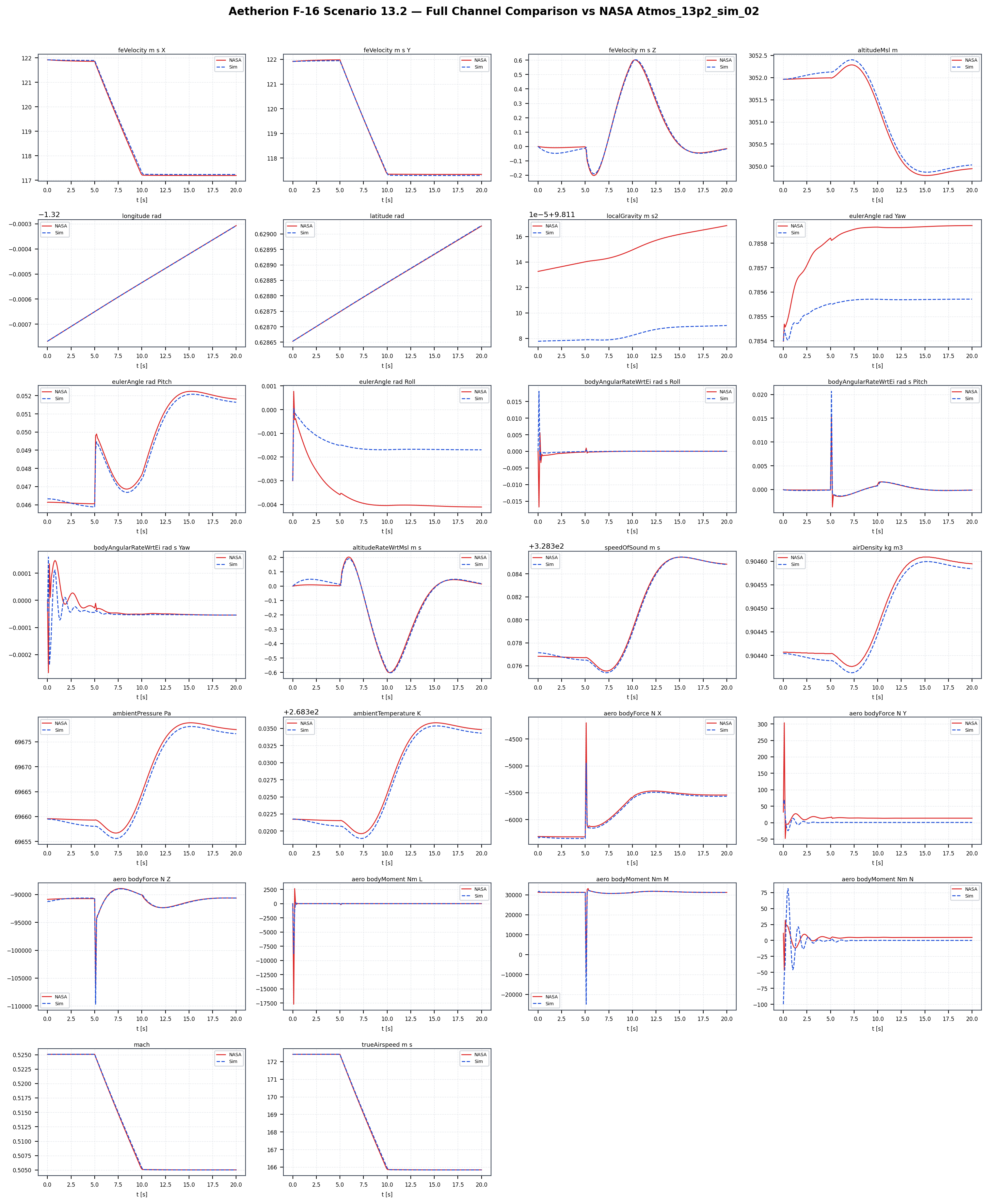
Scenario 13.2 simulation overview. Aetherion (blue dashed) vs NASA Atmos_13p2_sim_02 (red).
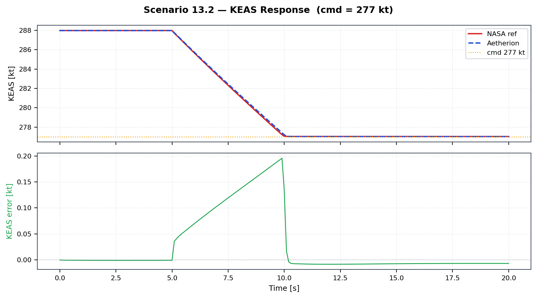
Scenario 13.2 KEAS response — commanded 277 kt (amber dotted), Aetherion (blue dashed), NASA ref (red). Final KEAS error < 0.01 kt.
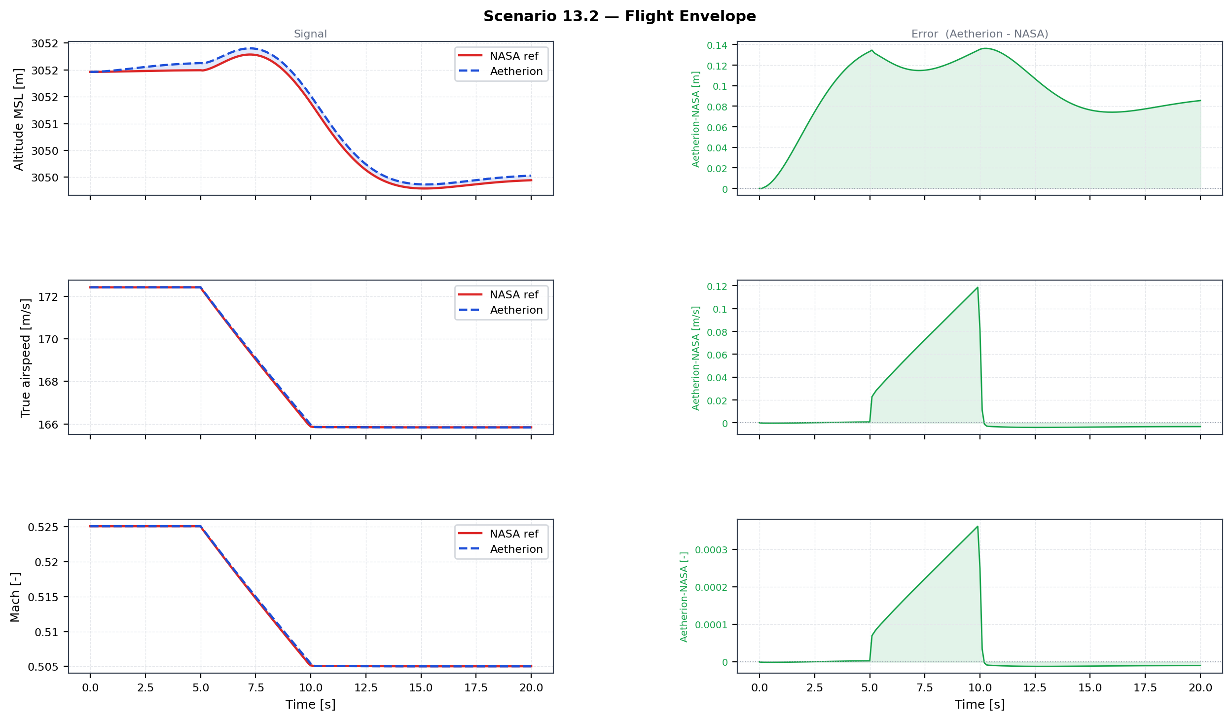
Scenario 13.2 flight envelope — altitude, TAS, Mach. Aetherion (blue dashed) vs NASA Atmos_13p2_sim_02 (red).
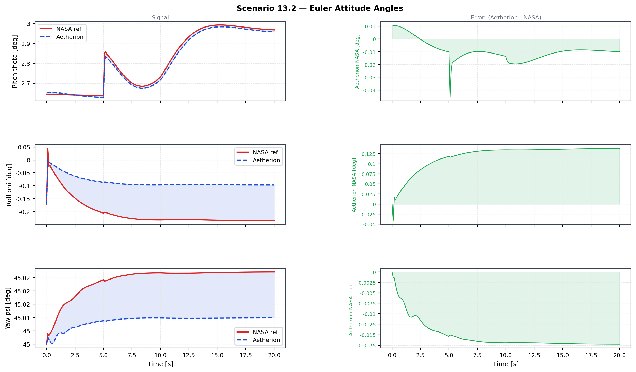
Scenario 13.2 Euler attitude angles — pitch, roll, yaw. Aetherion (blue dashed) vs NASA Atmos_13p2_sim_02 (red).
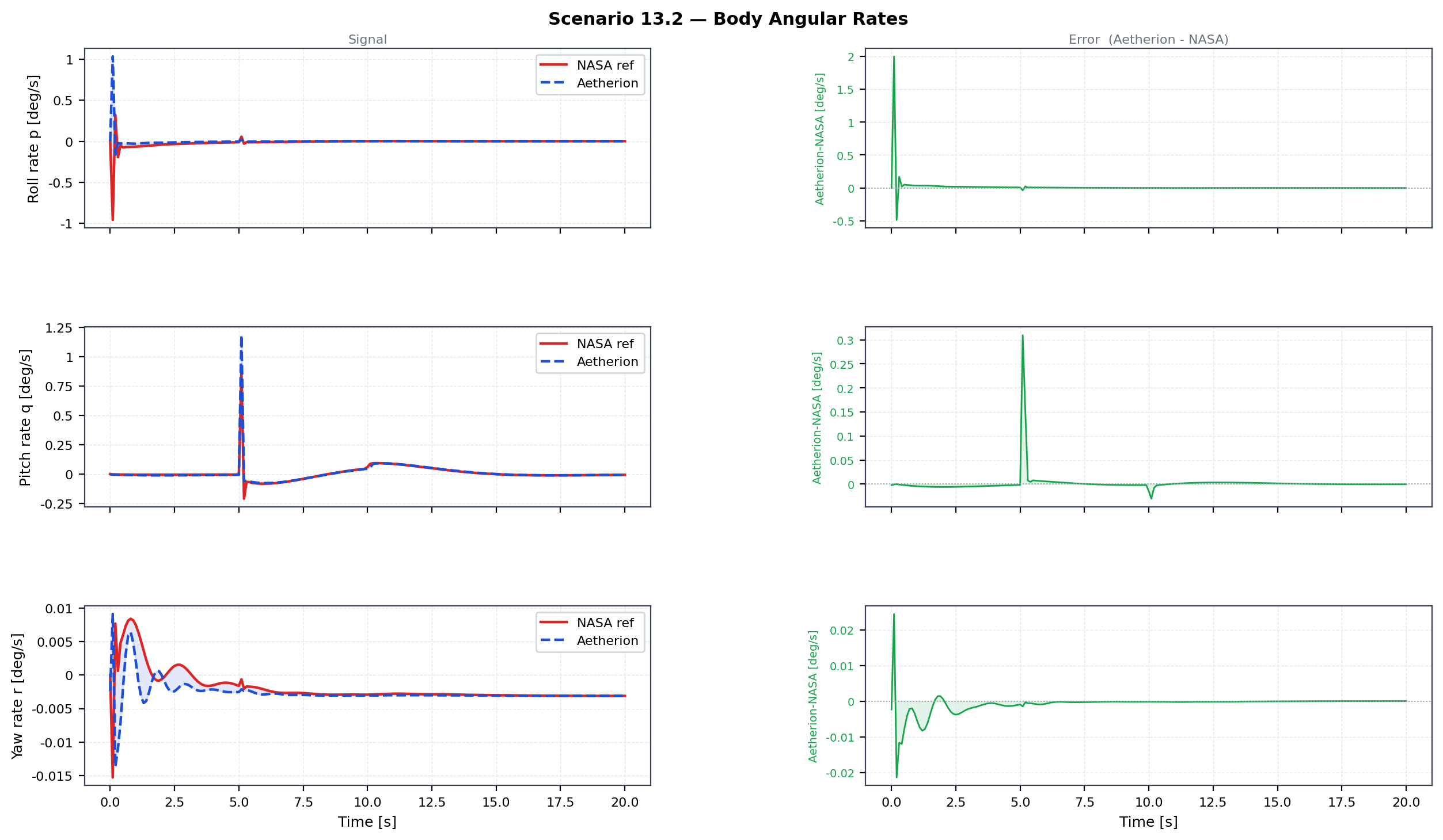
Scenario 13.2 body angular rates — roll, pitch, yaw rates. Aetherion (blue dashed) vs NASA Atmos_13p2_sim_02 (red).
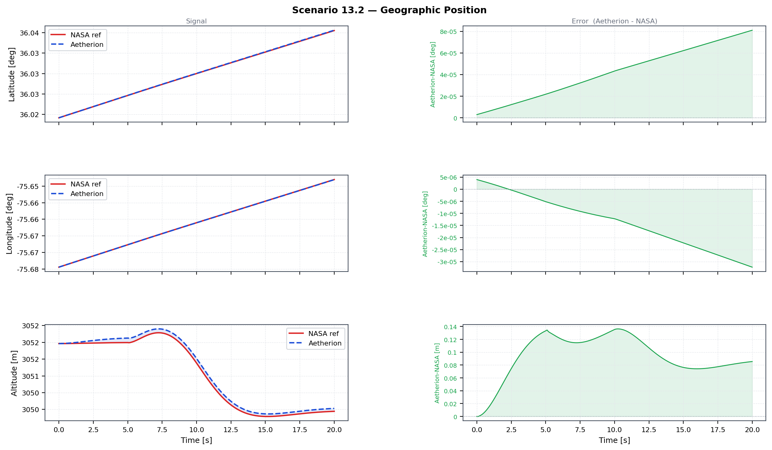
Scenario 13.2 geodetic position — altitude, latitude, longitude. Aetherion (blue dashed) vs NASA Atmos_13p2_sim_02 (red).
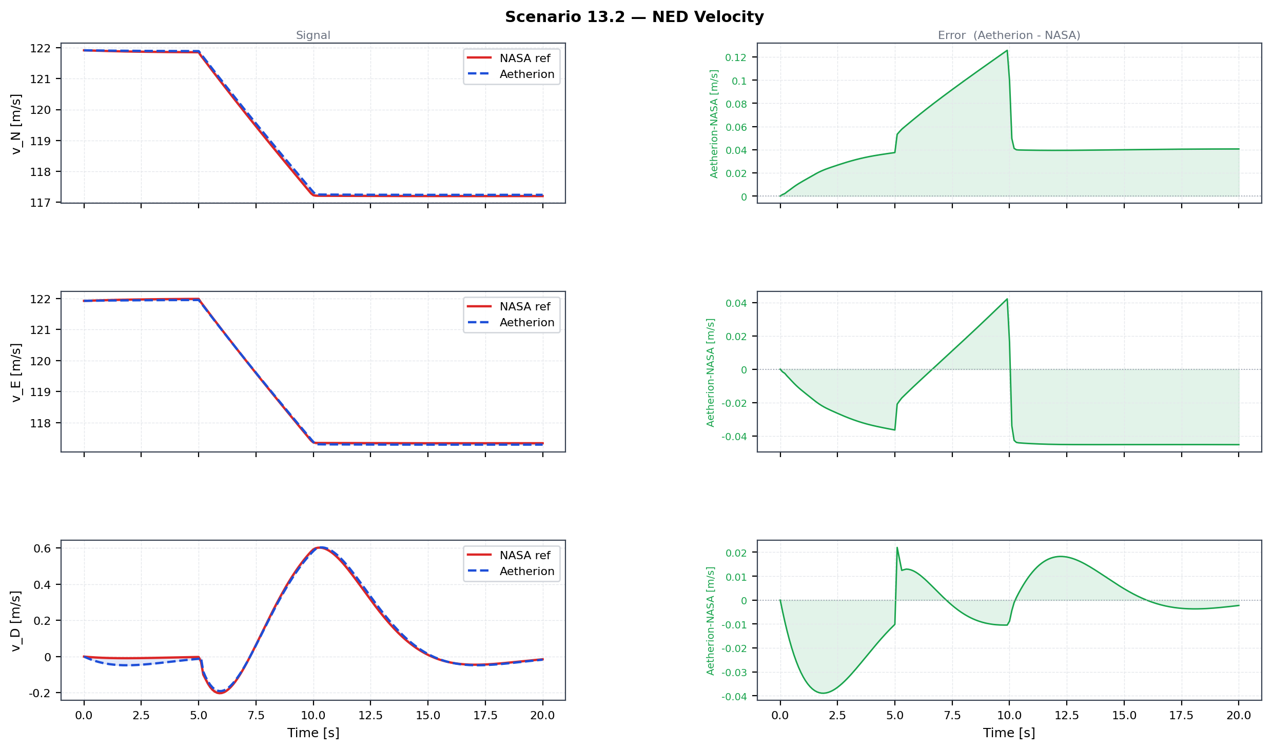
Scenario 13.2 NED velocity components — North, East, Down. Aetherion (blue dashed) vs NASA Atmos_13p2_sim_02 (red).
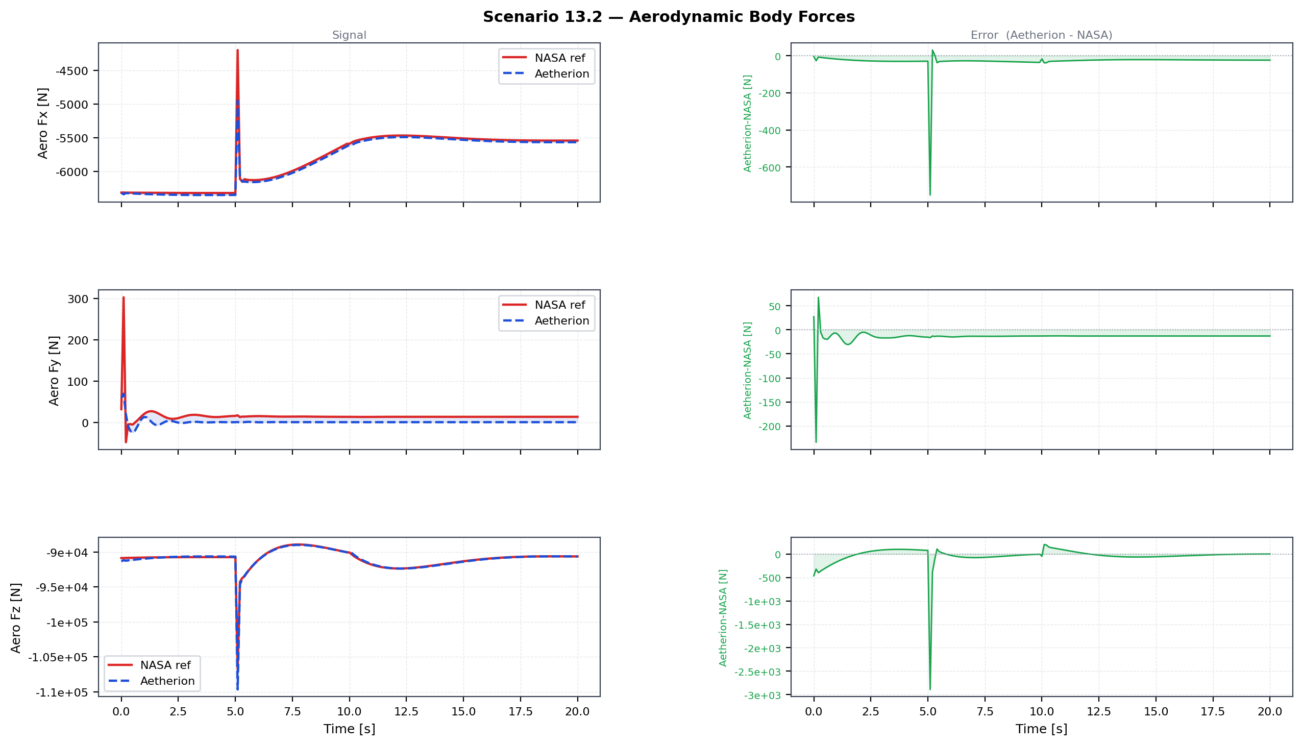
Scenario 13.2 aerodynamic body forces — X, Y, Z. Aetherion (blue dashed) vs NASA Atmos_13p2_sim_02 (red).
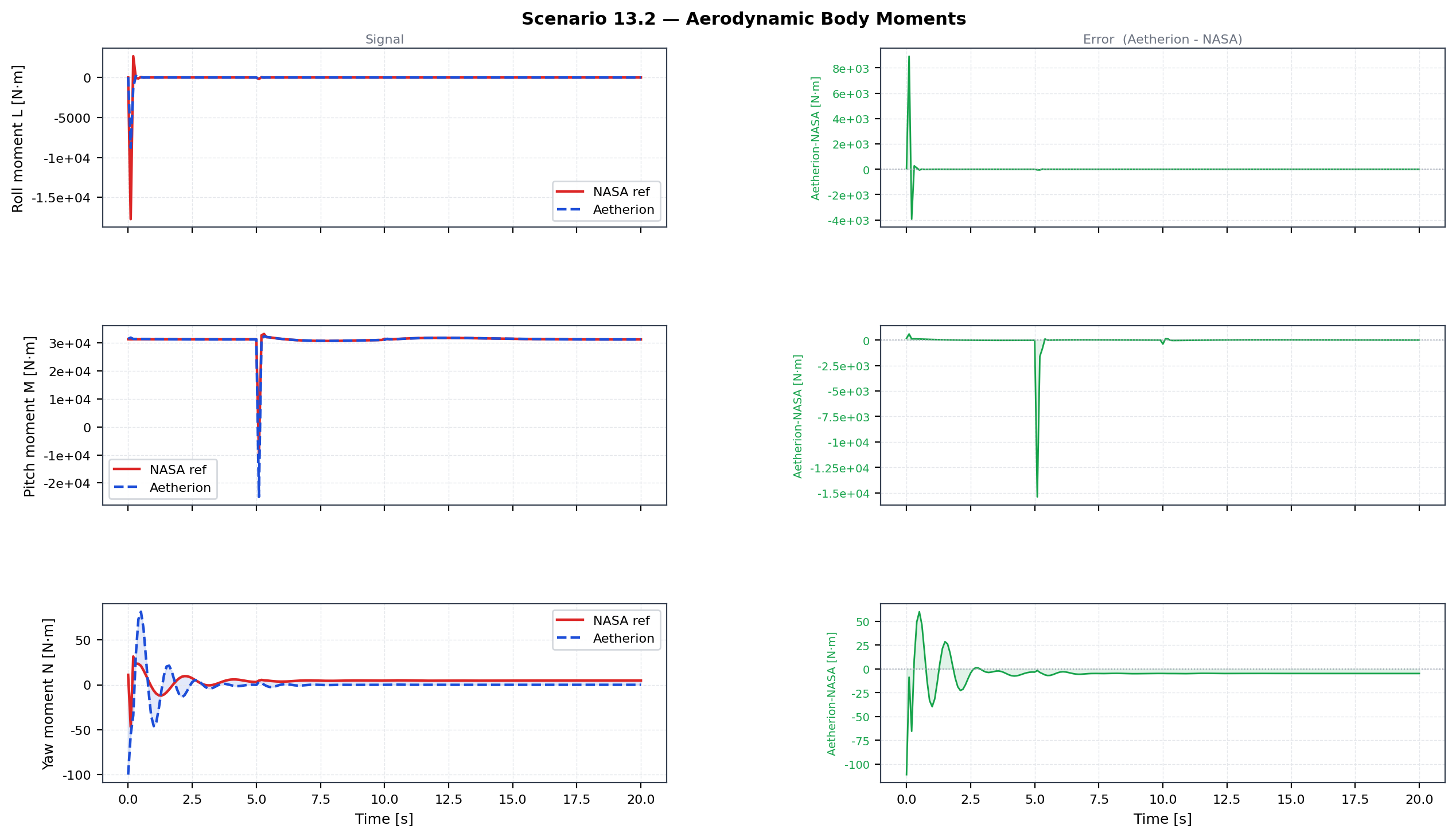
Scenario 13.2 aerodynamic body moments — L, M, N. Aetherion (blue dashed) vs NASA Atmos_13p2_sim_02 (red).
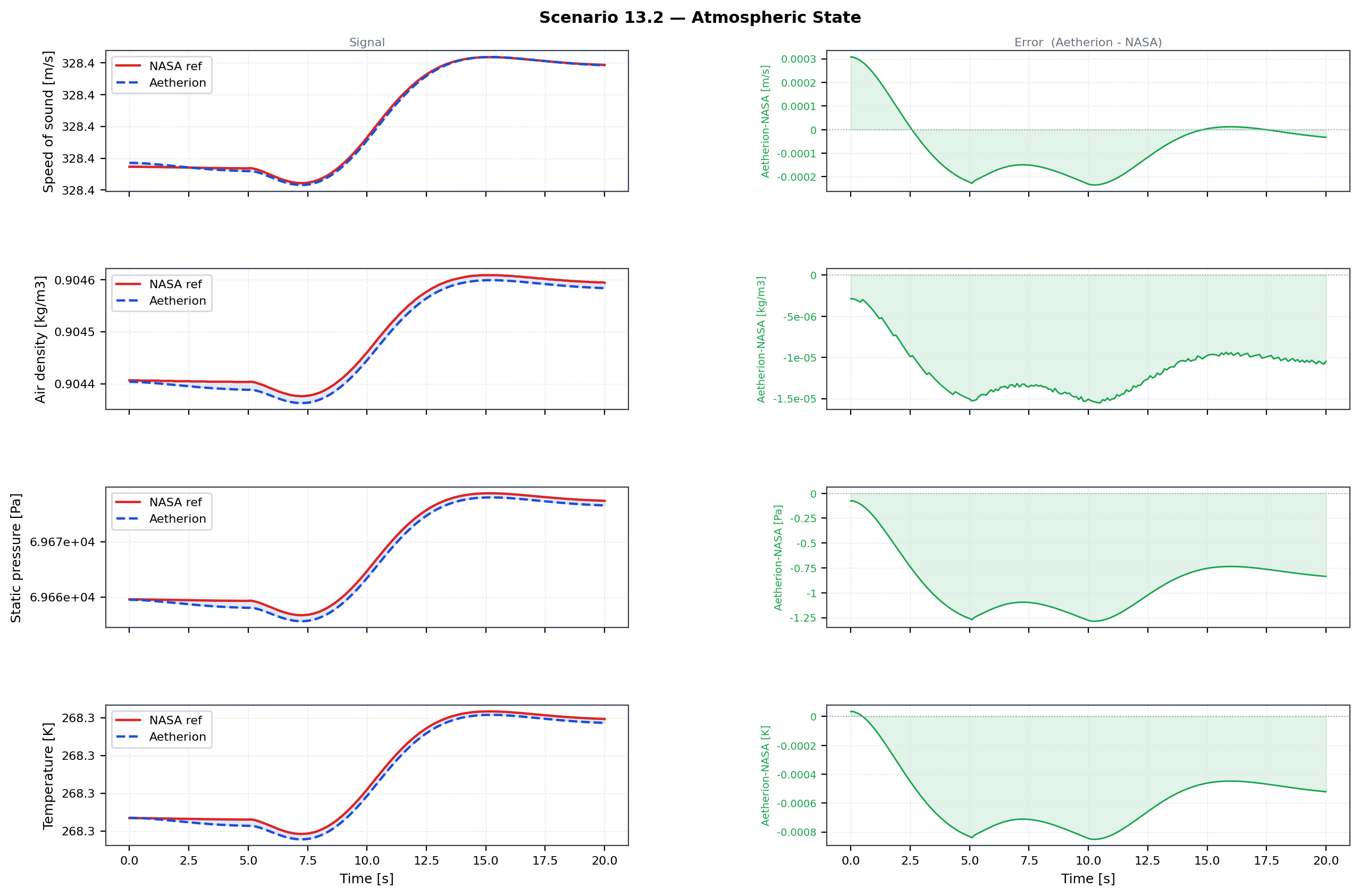
Scenario 13.2 atmosphere — temperature, density, pressure. Aetherion (blue dashed) vs NASA Atmos_13p2_sim_02 (red).
F-16 Subsonic Heading Change (NASA TM-2015-218675 Atmospheric Scenario 13.3)
Scenario overview
Starting from the same Kitty Hawk trim as Scenario 11, the F-16 executes
a closed-loop +15° course step (45° → 60° NE) driven by the NASA LQR SAS
and heading-hold autopilot defined in F16_control.dml.
The same two-loop GNC architecture and F16AltitudeChangeSimulator class are
reused unchanged. Only the autopilot commands differ:
Altitude command — hold 10 013 ft.
Airspeed command — hold trim KEAS (computed from US1976 atmosphere at the trim altitude so that
deltaVequiv ≈ 0at t = 0).Heading command — step from 45° to 60° applied at t = 15 s (NASA TM-2015-218675 Check-case 13.3: “At t = +15.0 sec, a 15° change in commanded heading to the right was made”). Before t = 15 s the controller holds the trim heading of 45°.
The DML heading autopilot estimates the track angle as
chiEst = beta + psi and computes
phi_cmd = −10 × (chiEst − chiCmd).
Applying the 15° step at t = 0 would immediately command
phi_cmd = +150°, causing a violent initial roll that does not match the
NASA reference. The chiStepTime_s field in F16AltitudeChangeCmds
enforces the correct t = 15 s timing.
The heading channel is driven by the lateral-directional LQR: a bank-angle command proportional to the course error causes the aircraft to roll into a coordinated turn and track the new heading.
Initial and command conditions
Parameter |
Value |
|---|---|
Location |
36.019° N, 75.674° W (Kitty Hawk, NC) |
Altitude (initial & commanded) |
10 013 ft (3 051.96 m) |
Heading (initial, held until t = 15 s) |
45° NE |
Heading command (baseChiCmd) |
60° (+15° step at t = 15 s) |
TAS (trim) |
335.15 KTAS (172.4 m/s) |
KEAS command |
computed from US1976 atmosphere at trim altitude (≈ 287.98 kt) |
Mach (trim) |
0.525 |
Simulation duration |
30 s |
Recommended run command
F16HeadingChange --endTime 30 --timeStep 0.02 \
                 --outputFileName f16_s13p3_sim.csv
The reference CSVs Atmos_13p3_sim_02/04/05.csv and the plot script
plot_f16_s13p3_nasa.py are copied to the build directory post-build.
Validation results at t = 30 s (dt = 0.02 s, chi step at t = 15 s)
Quantity |
Aetherion |
NASA sim 05 |
|---|---|---|
Altitude |
10 013.6 ft (3 052.1 m) |
10 013.3 ft (3 052.0 m) |
TAS |
172.42 m/s (335.16 kt) |
172.42 m/s (335.16 kt) |
Mach |
0.525075 |
0.525070 |
Yaw ψ |
59.92° |
59.92° |
Pitch θ |
2.627° |
2.627° |
Roll φ |
+0.82° |
+0.79° |
The final yaw agrees to within 0.003° of simulation 05, and altitude to 0.7 ft throughout. The peak errors — yaw ±2.5°, roll ±4.1° — last 0.6 s: the aircraft rolls into the turn at over 100 °/s, and the two zero-order-hold controllers sample the step at different instants. Against simulation 02 the same roll peak is 14°.
Validation figures
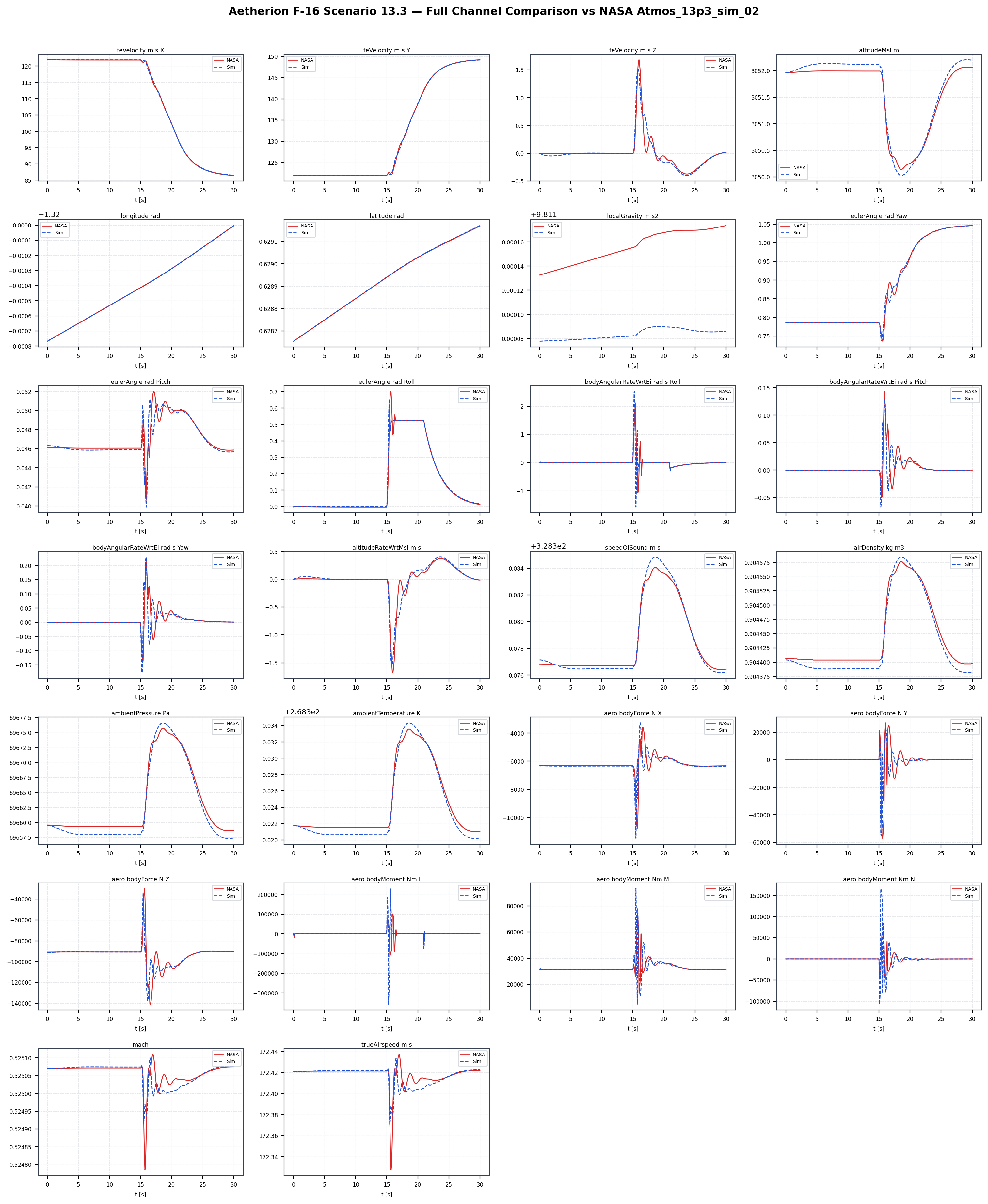
Scenario 13.3 simulation overview. Aetherion (blue dashed) vs NASA Atmos_13p3_sim_05 (red).
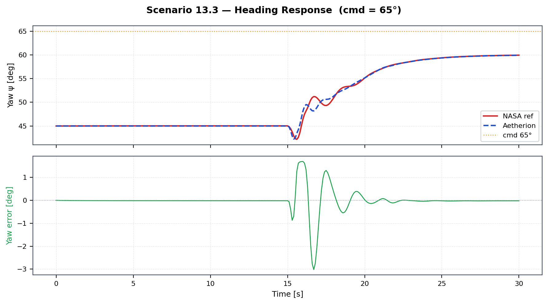
Scenario 13.3 heading (yaw) response — commanded 60° (amber dotted), Aetherion (blue dashed), NASA ref (red). Both settle to ≈ 59.9° at t = 30 s (Aetherion 59.92°, NASA ref 59.94°).
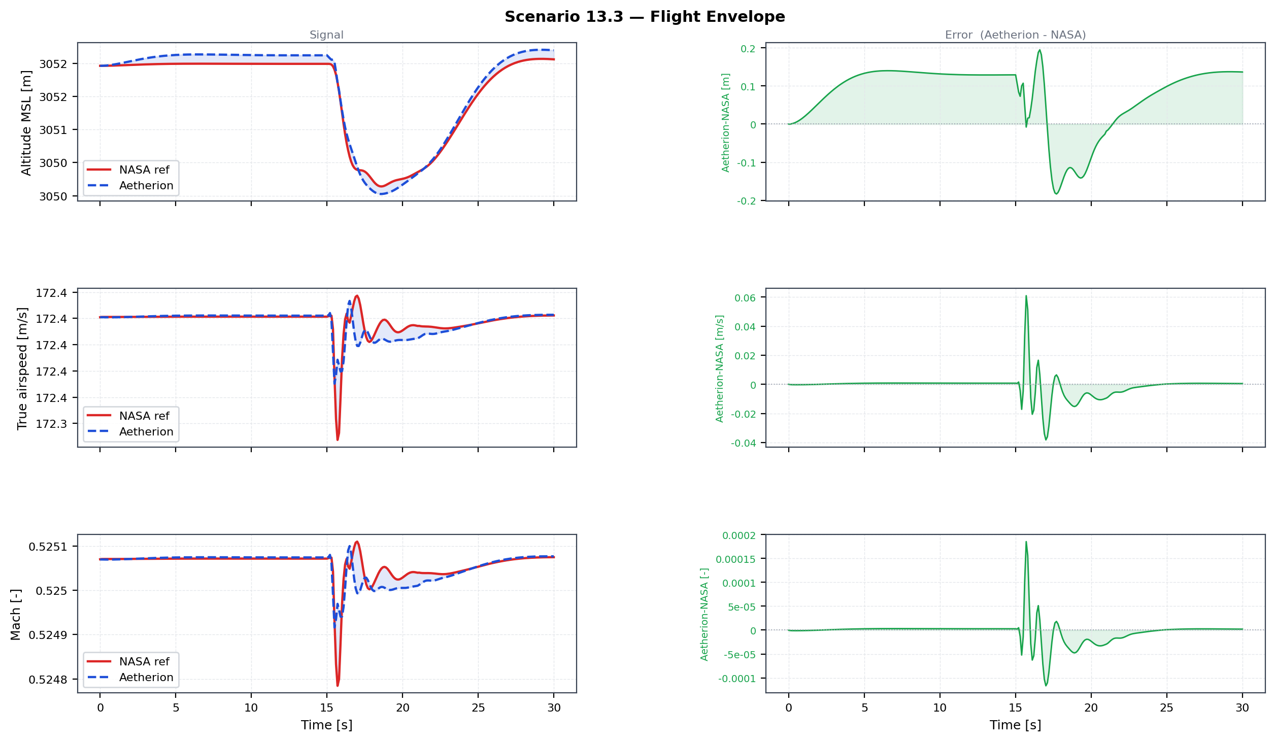
Scenario 13.3 flight envelope — altitude, TAS, Mach. Aetherion (blue dashed) vs NASA Atmos_13p3_sim_05 (red).
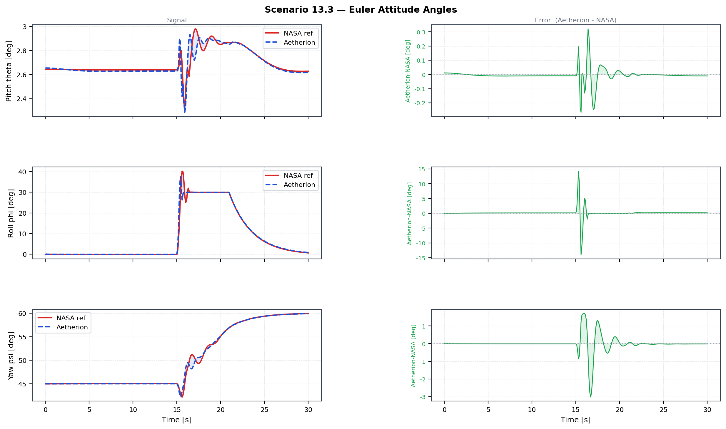
Scenario 13.3 Euler attitude angles — pitch, roll, yaw. Aetherion (blue dashed) vs NASA Atmos_13p3_sim_05 (red).
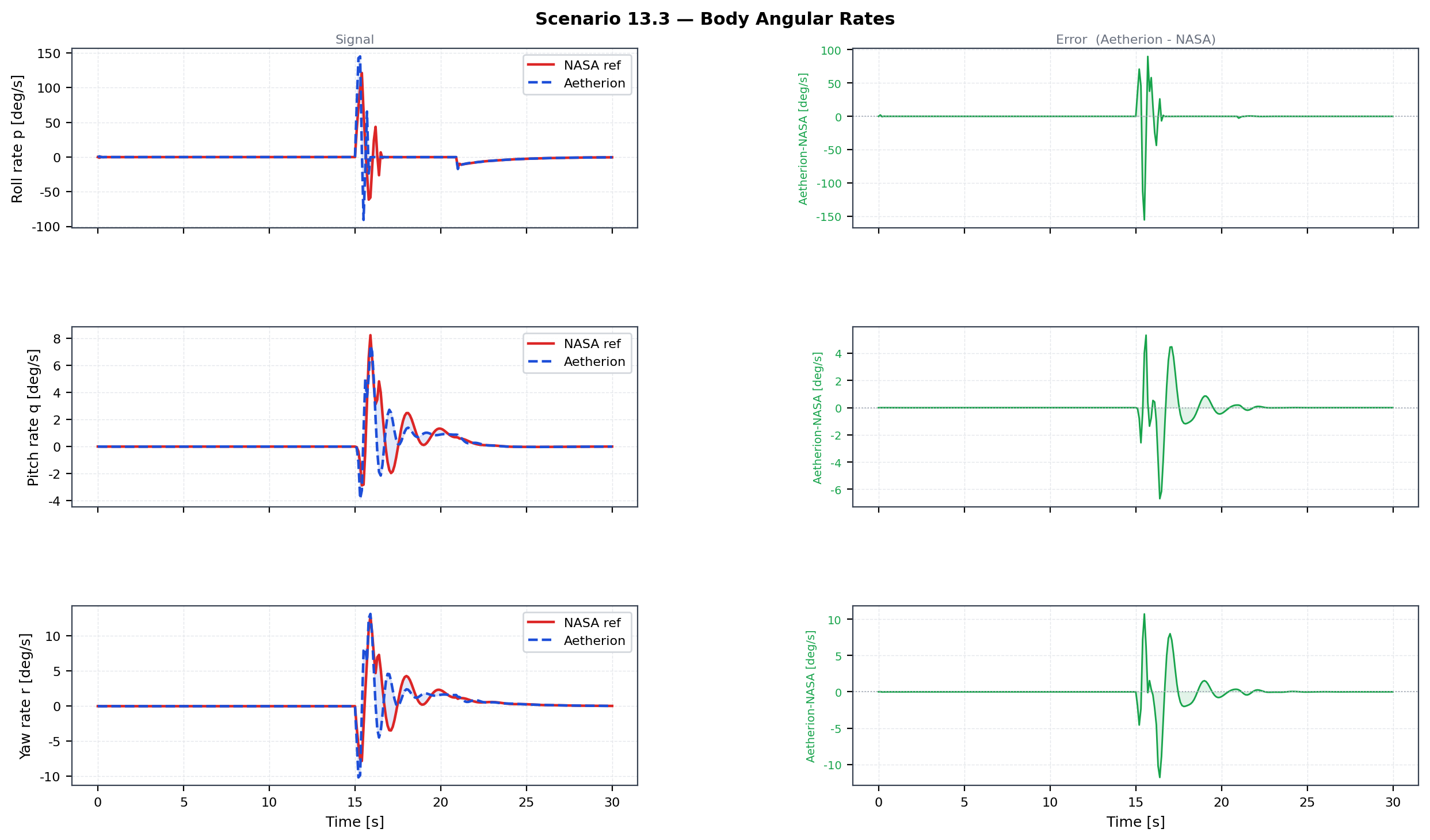
Scenario 13.3 body angular rates — roll, pitch, yaw rates. Aetherion (blue dashed) vs NASA Atmos_13p3_sim_05 (red).
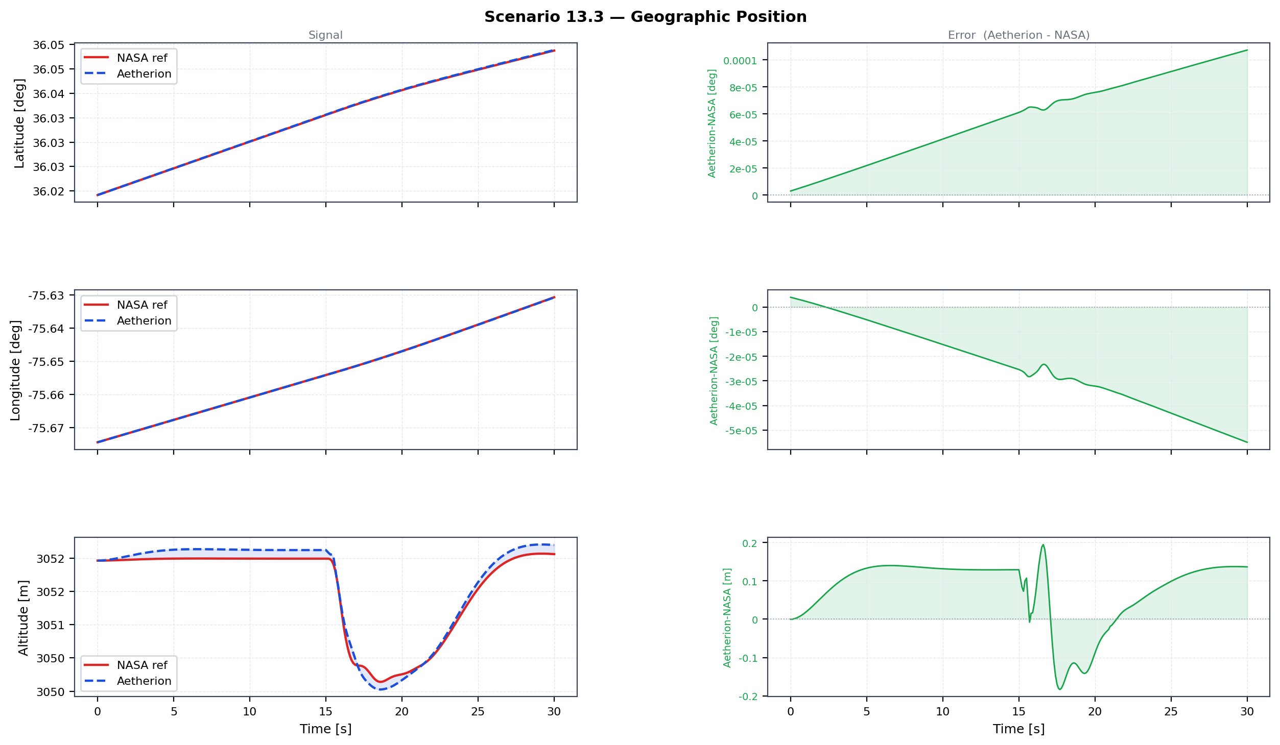
Scenario 13.3 geodetic position — altitude, latitude, longitude. Aetherion (blue dashed) vs NASA Atmos_13p3_sim_05 (red).
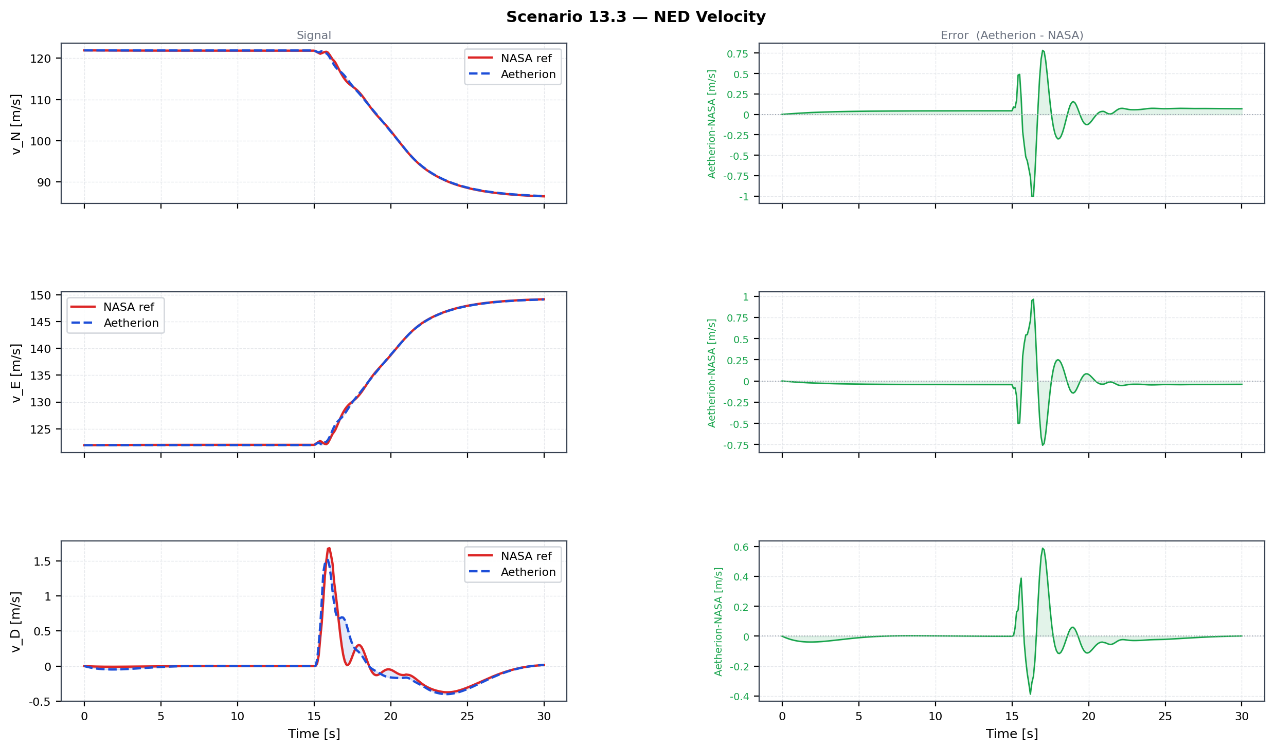
Scenario 13.3 NED velocity components — North, East, Down. Aetherion (blue dashed) vs NASA Atmos_13p3_sim_05 (red).
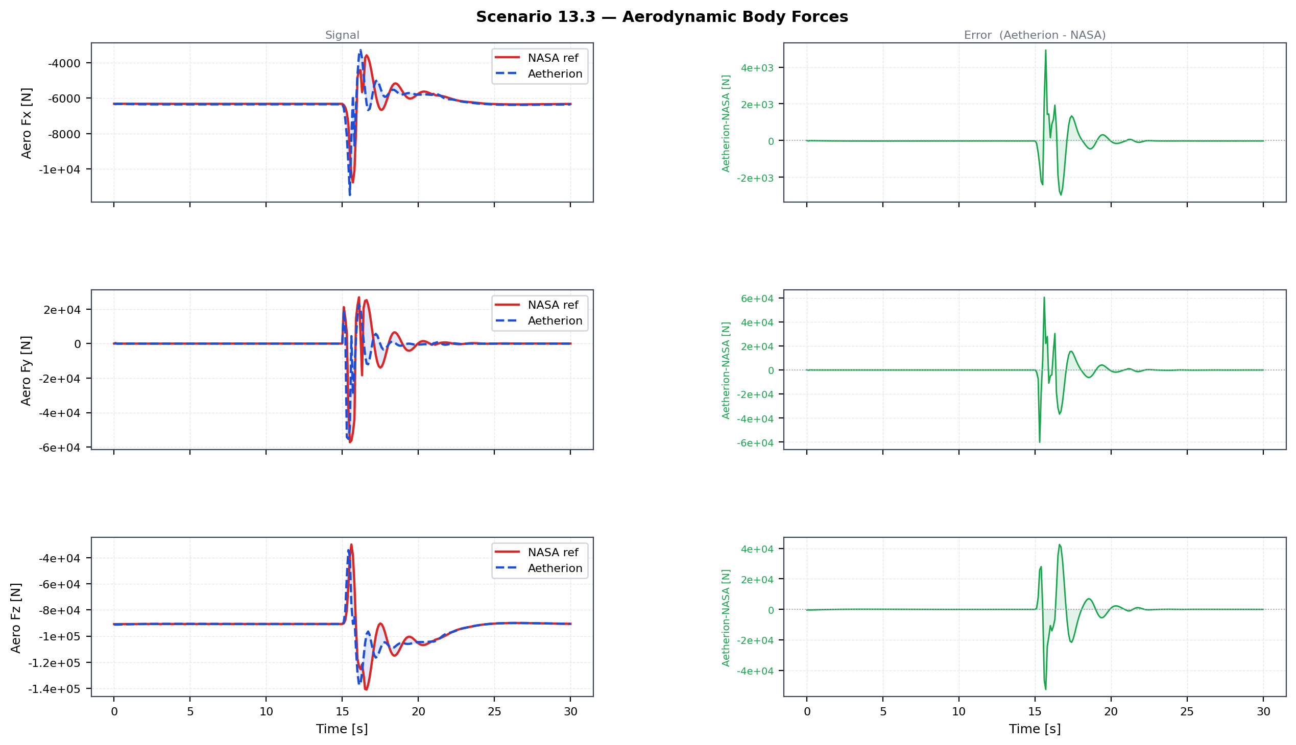
Scenario 13.3 aerodynamic body forces — X, Y, Z. Aetherion (blue dashed) vs NASA Atmos_13p3_sim_05 (red).
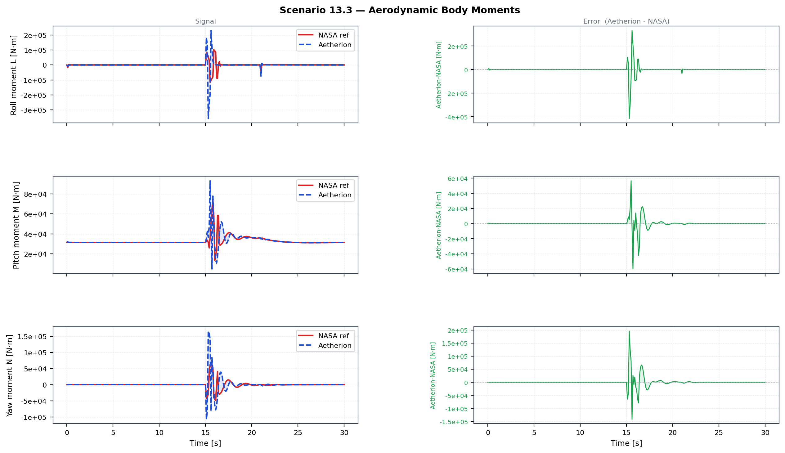
Scenario 13.3 aerodynamic body moments — L, M, N. Aetherion (blue dashed) vs NASA Atmos_13p3_sim_05 (red).
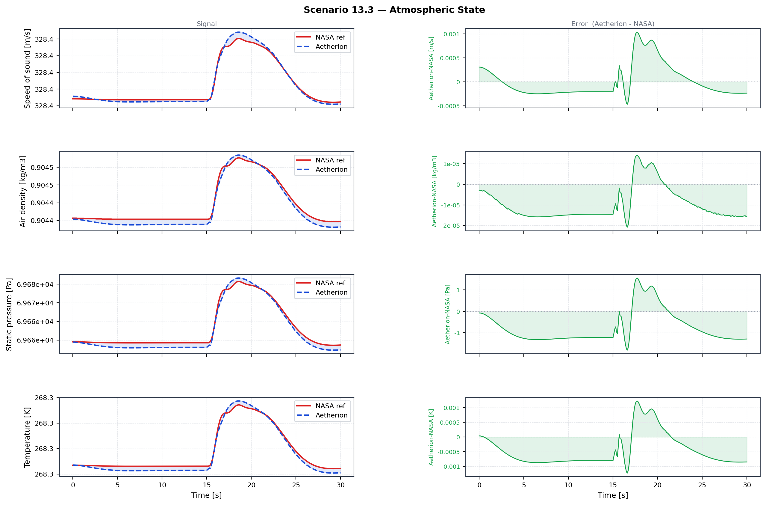
Scenario 13.3 atmosphere — temperature, density, pressure. Aetherion (blue dashed) vs NASA Atmos_13p3_sim_05 (red).
F-16 Subsonic Lateral Side Step (NASA TM-2015-218675 Atmospheric Scenario 13.4)
Scenario overview
Starting from the same Kitty Hawk trim as Scenario 11, the F-16 executes a
closed-loop 2 000 ft right-of-course lateral offset driven by the NASA
LQR SAS and lateral deviation autopilot defined in F16_control.dml.
The same two-loop GNC architecture and F16AltitudeChangeSimulator class are
reused. Only the autopilot commands differ:
Altitude command — hold 10 013 ft.
Airspeed command — hold trim KEAS throughout.
Heading command — hold 45° NE base course throughout.
Lateral offset — step from 0 ft to 2 000 ft right of the 45° NE courseline at t = 20 s (NASA TM-2015-218675 Check-case 13.4: “At t = +20.0 sec, a 2 000-ft lateral offset was commanded to the right”).
The lateralDeviationError fed to the DML control law is computed
dynamically at each integration step from the aircraft’s geodetic position
relative to the original 45° NE courseline, minus the commanded 2 000 ft
offset (applied after t = 20 s). This ensures the heading autopilot
commands a return to the new parallel track rather than continuing to turn.
The latStepTime_s / latStepOffset_ft fields in F16AltitudeChangeCmds
encode the step; the simulator recomputes latOffset_ft each step via
the latStepOffset_ft != 0 branch of extractFeedback().
Initial and command conditions
Parameter |
Value |
|---|---|
Location |
36.019° N, 75.674° W (Kitty Hawk, NC) |
Altitude (initial & commanded) |
10 013 ft (3 051.96 m) |
Heading command (base course) |
45° NE (held throughout) |
TAS (trim) |
335.15 KTAS (172.4 m/s) |
KEAS command |
computed from US1976 atmosphere at trim altitude (≈ 287.98 kt) |
Mach (trim) |
0.525 |
Lateral offset command |
2 000 ft right of course (applied at t = 20 s) |
Simulation duration |
60 s |
Recommended run command
F16LateralSideStep --endTime 60 --timeStep 0.02 \
                   --outputFileName f16_s13p4.csv
The reference CSVs Atmos_13p4_sim_02/04/05.csv and the plot script
plot_f16_s13p4_nasa.py are copied to the build directory post-build.
Validation results at t = 60 s (dt = 0.02 s, lat step at t = 20 s)
Quantity |
Aetherion |
NASA sim 05 |
|---|---|---|
Altitude |
10 013.3 ft (3 052.1 m) |
10 013.0 ft (3 052.0 m) |
TAS |
172.42 m/s (335.16 kt) |
172.42 m/s (335.16 kt) |
Mach |
0.5251 |
0.5251 |
Yaw ψ |
45.28° |
45.17° |
Roll φ |
−0.74° |
−0.72° |
Lateral deviation |
1 980 ft |
— |
The aircraft returns to within 0.28° of the base course heading at t = 60 s (simulation 05: 0.17°). Altitude stays within 6.5 ft of the commanded 10 013 ft through the manoeuvre, and within 0.7 ft of simulation 05. Peak errors during the turn entry: yaw ±2.3°, roll ±3.7° — 0.6 s of different zero-order-hold sampling while the aircraft rolls at over 100 °/s; against simulation 02 the same roll peak is 14°.
Validation figures
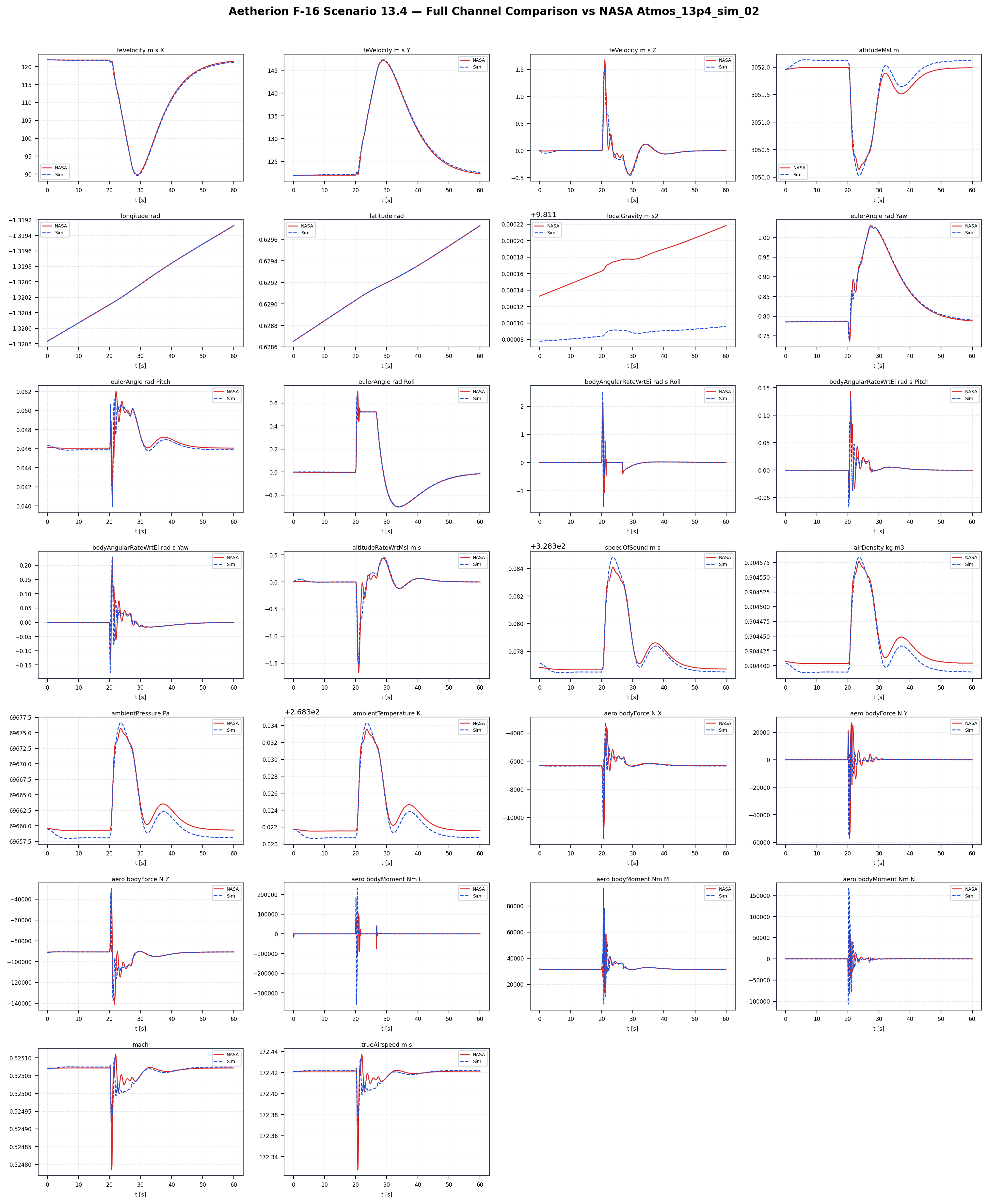
Scenario 13.4 simulation overview. Aetherion (blue dashed) vs NASA Atmos_13p4_sim_05 (red).
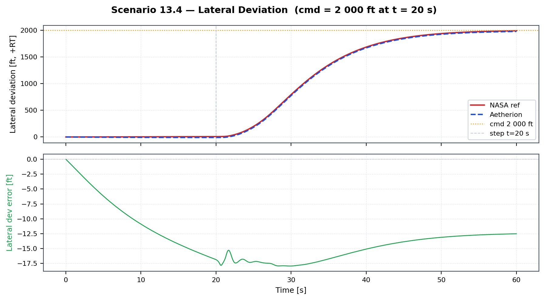
Scenario 13.4 lateral deviation response — commanded 2 000 ft offset (amber dotted), Aetherion (blue dashed), NASA ref (red).
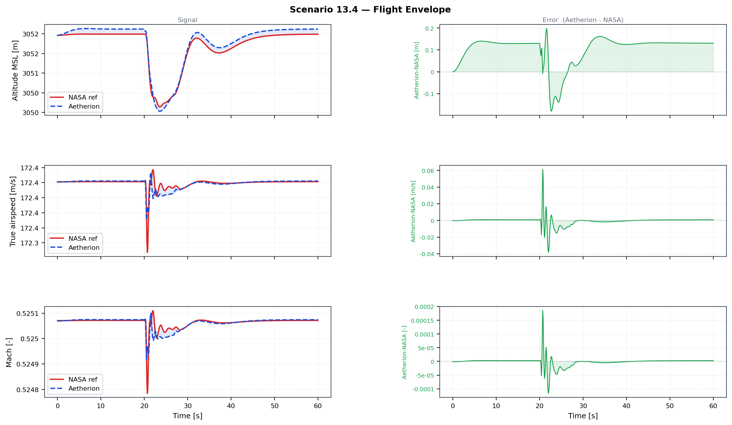
Scenario 13.4 flight envelope — altitude, TAS, Mach. Aetherion (blue dashed) vs NASA Atmos_13p4_sim_05 (red).
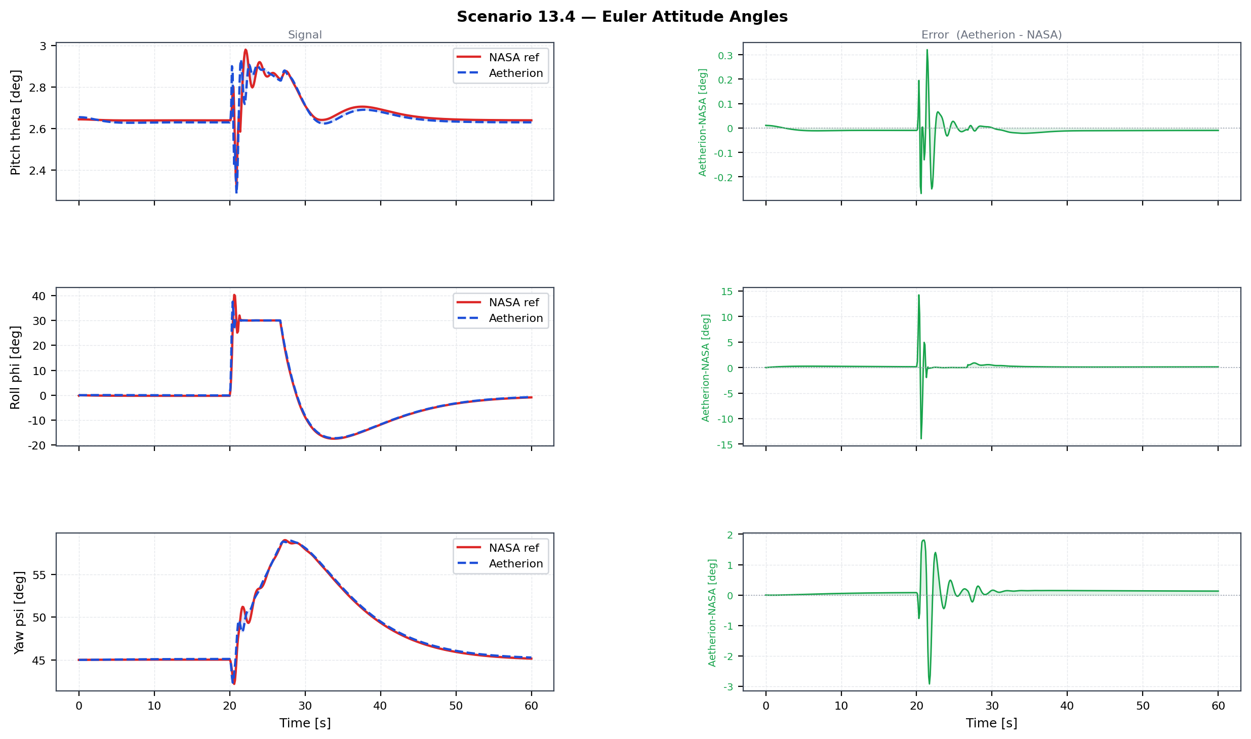
Scenario 13.4 Euler attitude angles — pitch, roll, yaw. Aetherion (blue dashed) vs NASA Atmos_13p4_sim_05 (red).
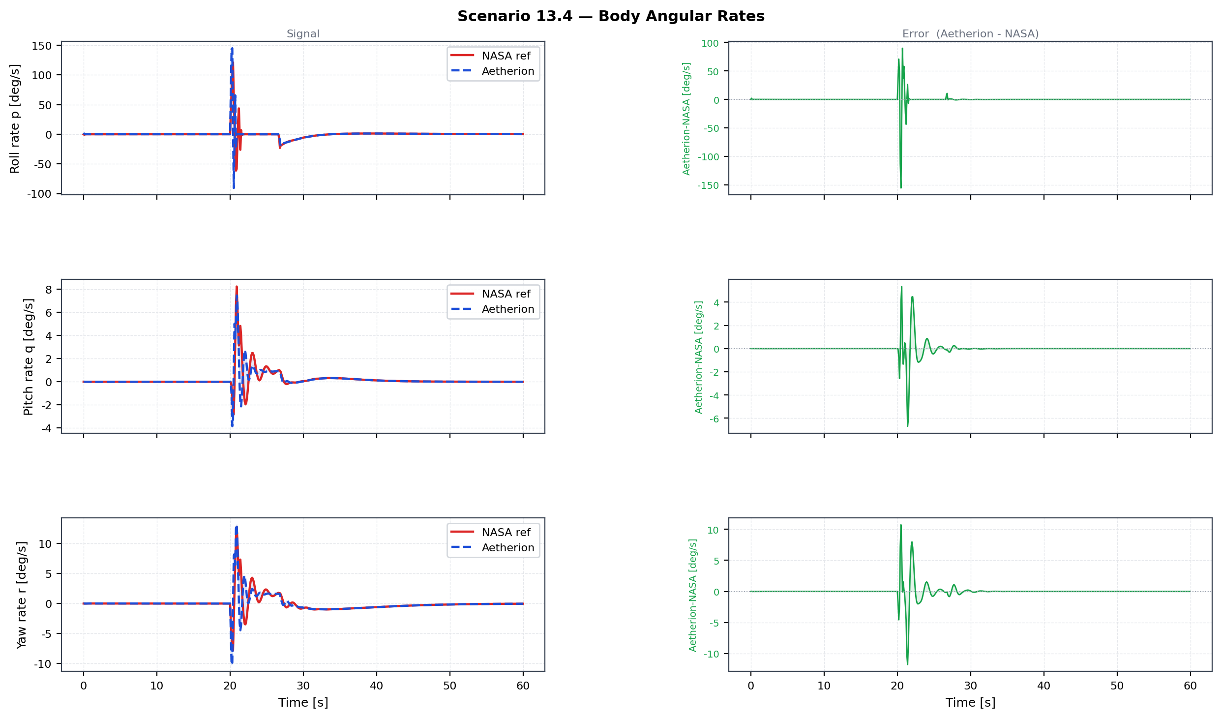
Scenario 13.4 body angular rates — roll, pitch, yaw rates. Aetherion (blue dashed) vs NASA Atmos_13p4_sim_05 (red).
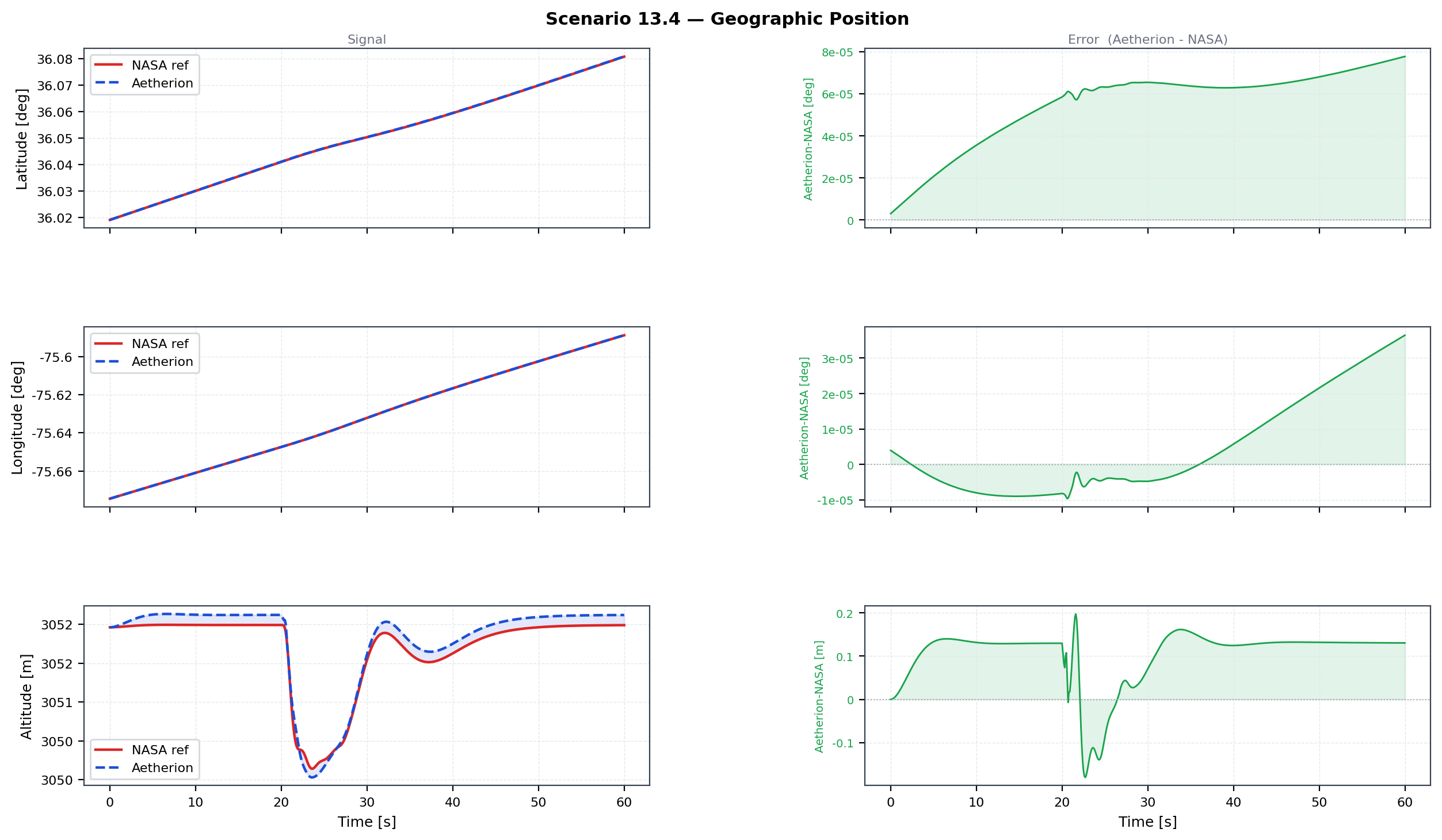
Scenario 13.4 geodetic position — altitude, latitude, longitude. Aetherion (blue dashed) vs NASA Atmos_13p4_sim_05 (red).
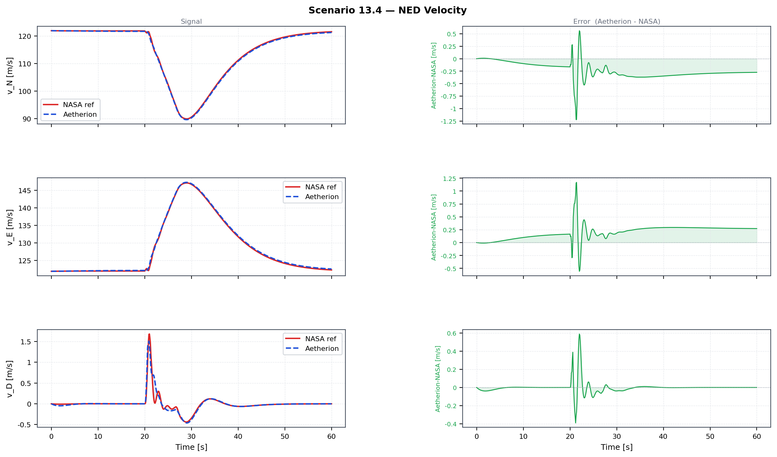
Scenario 13.4 NED velocity components — North, East, Down. Aetherion (blue dashed) vs NASA Atmos_13p4_sim_05 (red).
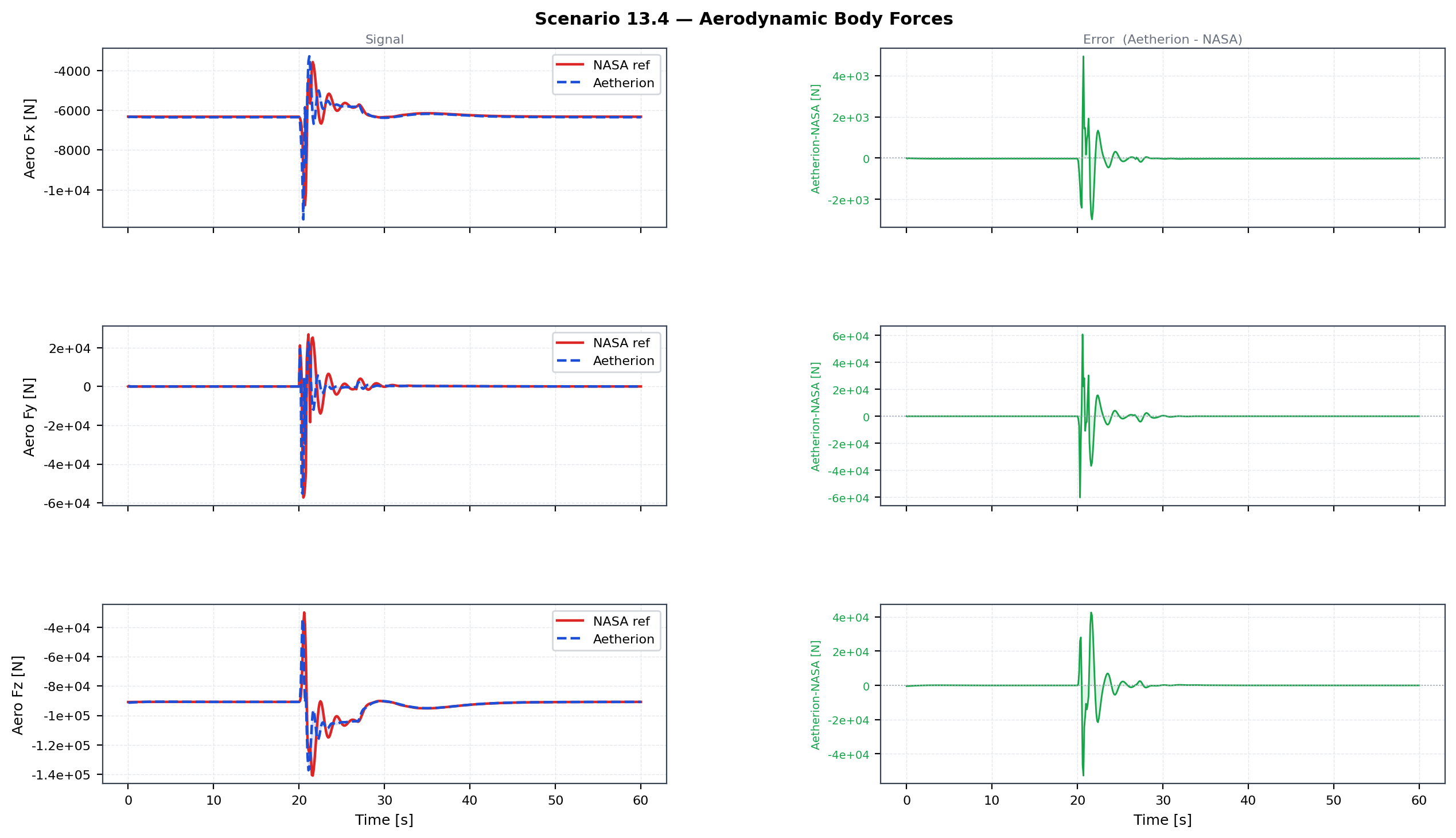
Scenario 13.4 aerodynamic body forces — X, Y, Z. Aetherion (blue dashed) vs NASA Atmos_13p4_sim_05 (red).
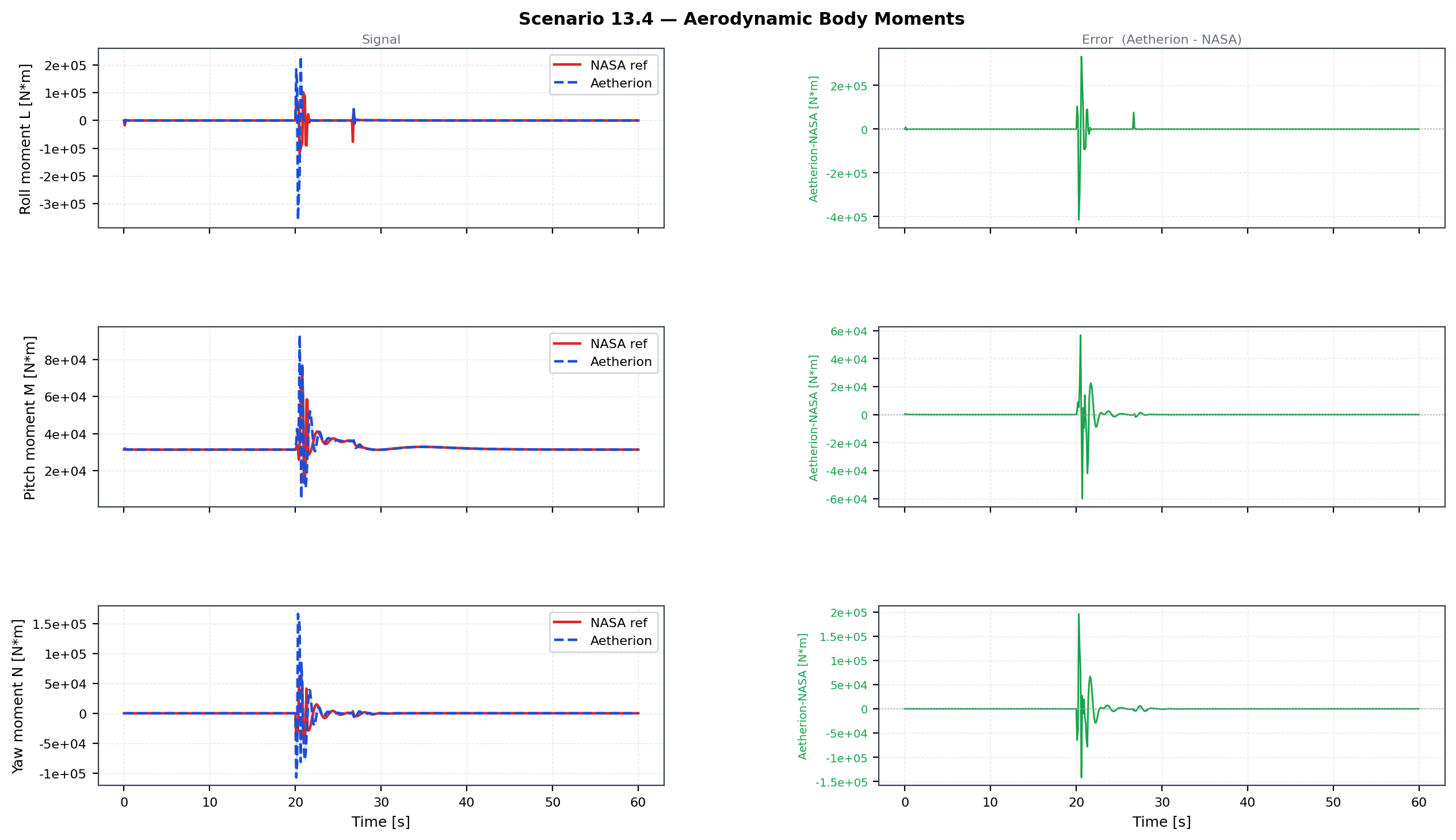
Scenario 13.4 aerodynamic body moments — L, M, N. Aetherion (blue dashed) vs NASA Atmos_13p4_sim_05 (red).
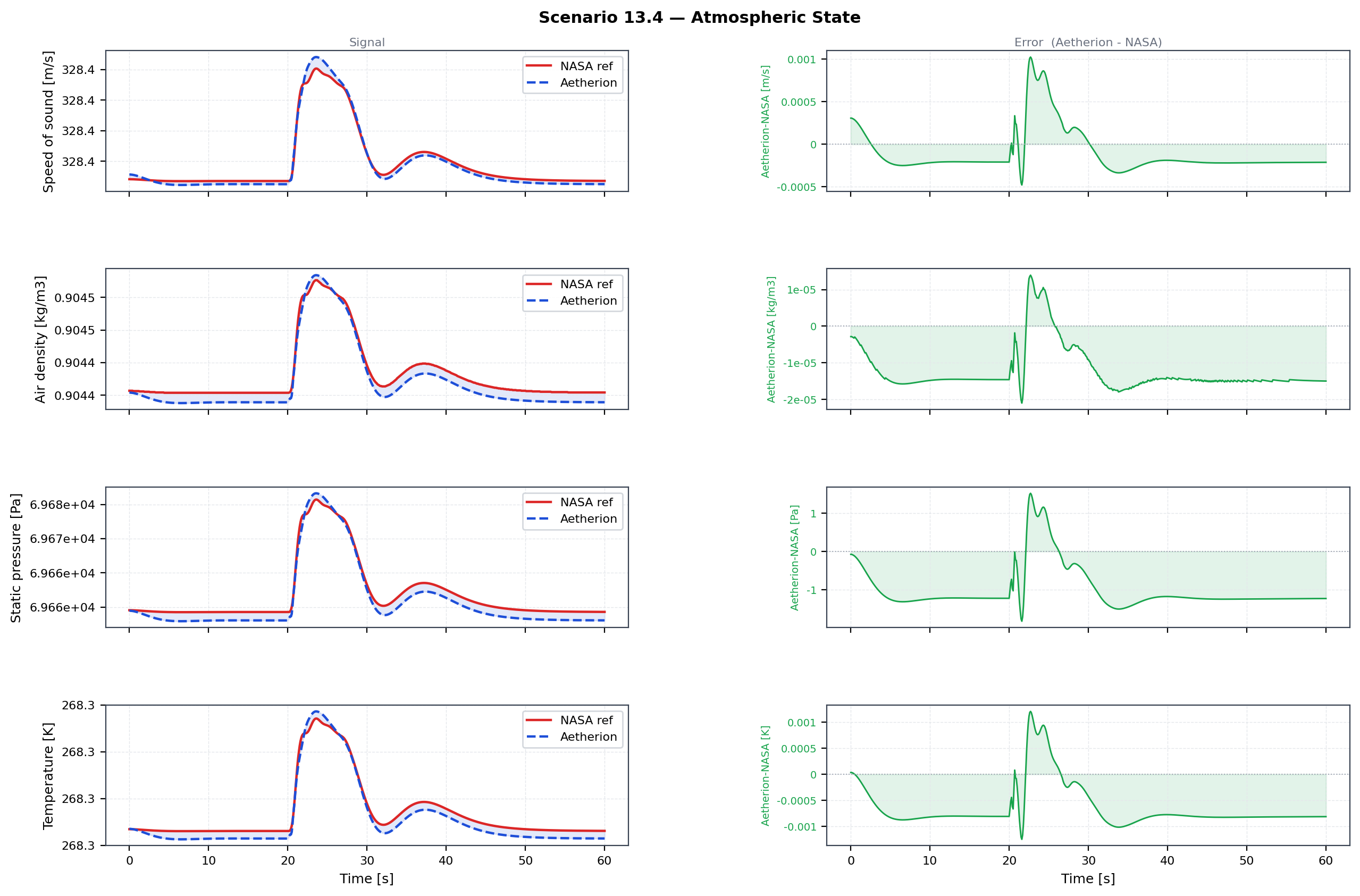
Scenario 13.4 atmosphere — temperature, density, pressure. Aetherion (blue dashed) vs NASA Atmos_13p4_sim_05 (red).
F-16 North Pole Circumnavigation (NASA TM-2015-218675 Atmospheric Scenario 15)
Scenario overview
This scenario tests the most demanding geodetic edge case in the NASA reference: a full six-DOF F-16 simulation that circumnavigates the geographic North Pole on a 3-nautical-mile-radius circular track. Two distinct challenges are exercised simultaneously:
Polar singularity — at lat ≈ 90° the factor \(\cos\phi\) in the longitude rate equation approaches zero, so a tiny change in body heading produces a very large change in geodetic longitude.
Antimeridian crossing — the vehicle repeatedly crosses ±180° geodetic longitude; the control system must wrap longitude correctly rather than treating the jump as a large position error.
The control model is ``F16_gnc.dml`` — a superset of F16_control.dml
that adds a circumnavigator outer loop. Setting the selectCircumnavigator
discrete input to 1.0 activates this loop: the DML model computes the
required bank-angle command to fly a steady 3-nmi left-hand circle centred on
the North Pole, with altitude and airspeed holds active throughout.
The GNC inputs ownshipN_deg (geodetic latitude) and ownshipE_deg
(geodetic longitude) are computed from the ECI state inside
F16AltitudeChangeSimulator::extractFeedback() and passed to the DML model
at every integration step.
The vehicle is trimmed straight and level at 10 000 ft / 563.6 ft/s TAS (Mach 0.523) before the simulation starts; the circumnavigating autopilot is engaged from the very first time step. Within approximately 30 s the aircraft has intercepted the desired circular track and settles into a steady left bank of ≈ 28°.
Circle geometry
The 3-nmi radius from the North Pole corresponds to a geodetic latitude of:
At this latitude the track circumference is:
At the trim TAS of 171.8 m/s (563.6 ft/s) the nominal circuit period is:
The 180-second run therefore covers approximately 311° of the full circle (the first ~30 s are spent intercepting the circular track from the initial heading-east condition; the remaining 150 s are at steady state).
Steady-state bank angle
For a coordinated level turn at radius \(R\) and true airspeed \(V\):
The NASA reference CSV confirms roll ≈ −28° at steady state (t ≥ 60 s).
Initial and command conditions
Parameter |
Value |
|---|---|
Location |
89.950° N, 45.000° W (near geographic North Pole) |
Altitude (initial & commanded) |
10 000 ft (3 048.0 m) |
Heading (initial) |
90° east |
TAS (trim) |
563.643 ft/s ≈ 333.95 kt (Mach 0.523) |
KEAS command |
computed from US1976 atmosphere at 10 000 ft |
Autopilot: |
1.0 (circumnavigator ON from t = 0) |
Geodesy / gravity |
WGS-84 rotating ellipsoid, J₂ gravity |
Atmosphere |
US Standard Atmosphere 1976, no wind |
Simulation duration |
180 s |
Trim result
The trim conditions at 10 000 ft / 563.643 ft/s TAS are identical to those of Scenario 11 scaled to the lower altitude (same aircraft, same atmosphere):
Quantity |
Aetherion |
NASA ref |
|---|---|---|
α (trim) |
2.689° |
2.689° |
δe (trim) |
≈ −3.24° |
— |
Throttle (trim) |
≈ 13.9 % |
— |
Recommended run command
CircleNorthPole --endTime 180 --timeStep 0.02 \
                --outputFileName atmos_15_output.csv
The reference CSVs Atmos_15_sim_02/04/05.csv are copied to the build
directory post-build.
Validation results (NASA reference Atmos_15_sim_05)
The table below shows the NASA reference trajectory at selected time steps. The vehicle intercepts the circle track by t ≈ 30 s and sustains steady-state circumnavigation (constant altitude, roll, and TAS) for the remaining 150 s.
\(t\) [s] |
Alt [ft] |
Lat [°] |
Lon [°] |
Yaw [°] |
Pitch [°] |
Roll [°] |
Mach |
|---|---|---|---|---|---|---|---|
0 |
10 000.00 |
89.9500 |
−45.000 |
90.00 |
2.687 |
0.000 |
0.5231 |
30 |
9 994.28 |
89.9486 |
+6.889 |
88.26 |
2.861 |
−29.996 |
0.5231 |
60 |
9 994.93 |
89.9488 |
+58.449 |
88.57 |
2.839 |
−28.027 |
0.5231 |
90 |
9 994.91 |
89.9488 |
+110.075 |
88.59 |
2.840 |
−28.077 |
0.5231 |
120 |
9 994.91 |
89.9488 |
+161.701 |
88.59 |
2.840 |
−28.077 |
0.5231 |
150 |
9 994.91 |
89.9488 |
−146.673 |
88.59 |
2.840 |
−28.077 |
0.5231 |
180 |
9 994.91 |
89.9488 |
−95.046 |
88.59 |
2.840 |
−28.077 |
0.5231 |
Key observations from the reference trajectory:
Altitude holds within 6 ft of the commanded 10 000 ft after the initial transient, confirming the altitude-hold autopilot is functioning.
Bank angle stabilises at −28.1° (left bank) from t ≈ 60 s onward, consistent with the analytical prediction of −28.3° for a 3-nmi radius turn.
Longitude advances by ≈ 51.6° per 30 s at steady state (longitude rate ≈ 1.72°/s), equivalent to a ~209-second orbital period and a ground-track of 34 900 m per circuit.
The vehicle crosses the antimeridian (±180°) between t = 120 s and t = 150 s without any discontinuity in the physical trajectory, confirming correct longitude wrapping in the geodetic conversion.
Latitude stabilises at 89.9488° (≈ 0.0012° equatorward of the initial 89.950°), consistent with the circumnavigator settling on the desired 3-nmi track (a shift of ≈ 134 m from the initial position).
Aetherion simulation results
The table below compares Aetherion against the NASA reference at selected time steps. The simulation matches the reference within normal numerical tolerance at all checkpoints.
\(t\) [s] |
Alt [ft] |
Lat [°] |
Lon [°] |
Yaw [°] |
Pitch [°] |
Roll [°] |
Mach |
|---|---|---|---|---|---|---|---|
0 |
10 000.00 |
89.9500 |
−45.000 |
90.00 |
2.687 |
0.000 |
0.5231 |
30 |
9 994.26 |
89.9486 |
+6.884 |
88.30 |
2.862 |
−29.995 |
0.5231 |
60 |
9 994.91 |
89.9488 |
+58.436 |
88.57 |
2.840 |
−28.042 |
0.5231 |
90 |
9 994.89 |
89.9488 |
+110.061 |
88.59 |
2.841 |
−28.098 |
0.5231 |
120 |
9 994.89 |
89.9488 |
+161.686 |
88.59 |
2.841 |
−28.099 |
0.5231 |
150 |
9 994.89 |
89.9488 |
−146.688 |
88.59 |
2.841 |
−28.099 |
0.5231 |
180 |
9 994.89 |
89.9488 |
−95.063 |
88.59 |
2.841 |
−28.099 |
0.5231 |
Against simulation 05 the maximum latitude error is 0.000017° (2 m) and the maximum longitude error 0.0164° over the whole trajectory; altitude agrees to 0.10 ft. Roll agrees to 0.02° from t = 60 s onward (0.6° peak while the circle is being captured), and altitude is held within 5.7 ft of 10 000 ft from t = 30 s onward.
Validation figures
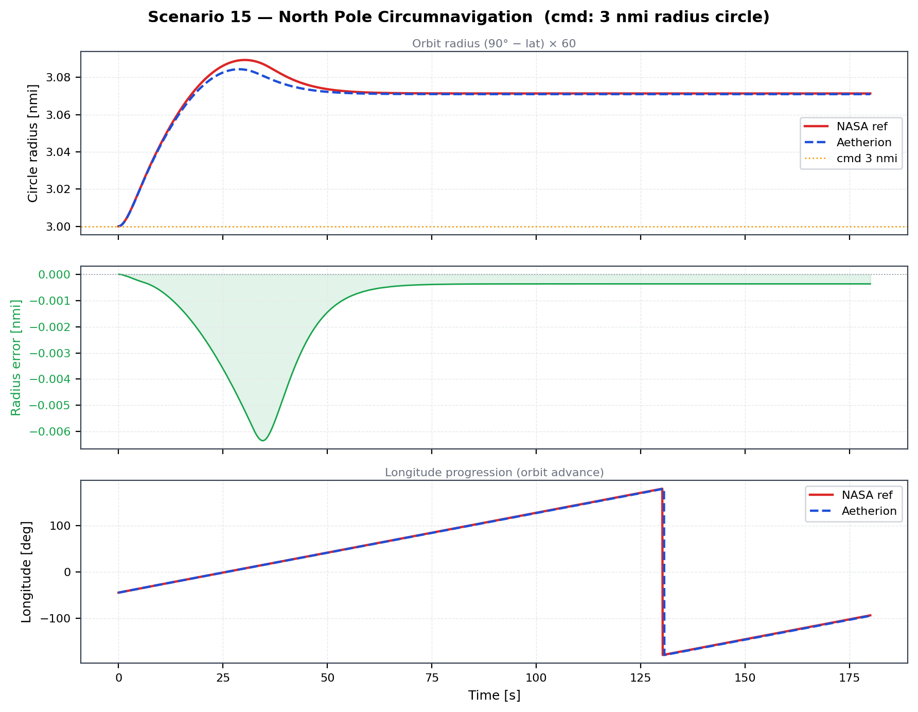
Scenario 15 orbit radius (top) and longitude progression (bottom). The circumnavigator holds the aircraft within < 0.003 nmi of the commanded 3-nmi circle from t ≈ 30 s onward. Aetherion (blue dashed) vs NASA Atmos_15_sim_05 (red).
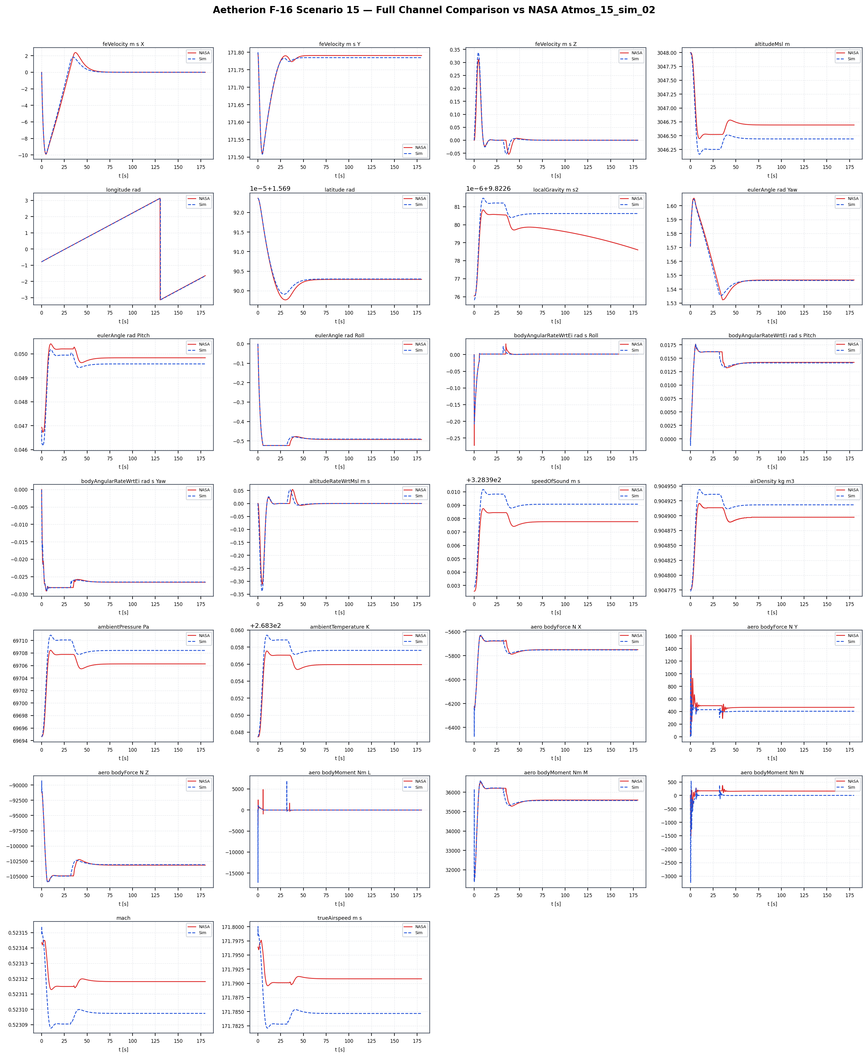
Scenario 15 simulation overview — 180 s north-pole circumnavigation. Aetherion (blue dashed) vs NASA Atmos_15_sim_05 (red).
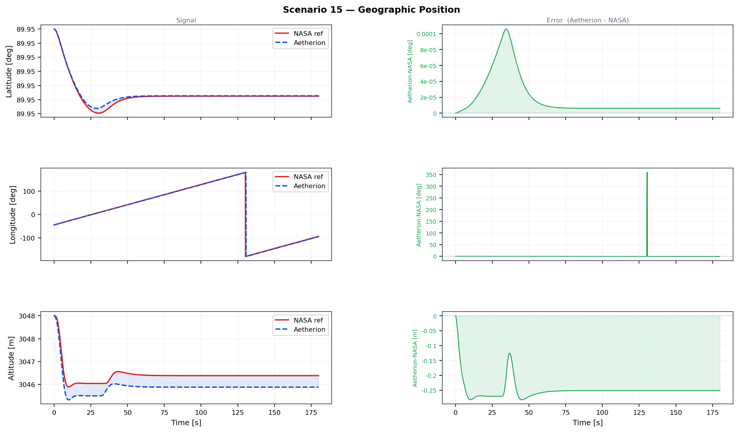
Scenario 15 geodetic position — altitude, latitude, and longitude (note the antimeridian crossing near t = 135 s). Aetherion (blue dashed) vs NASA Atmos_15_sim_05 (red).
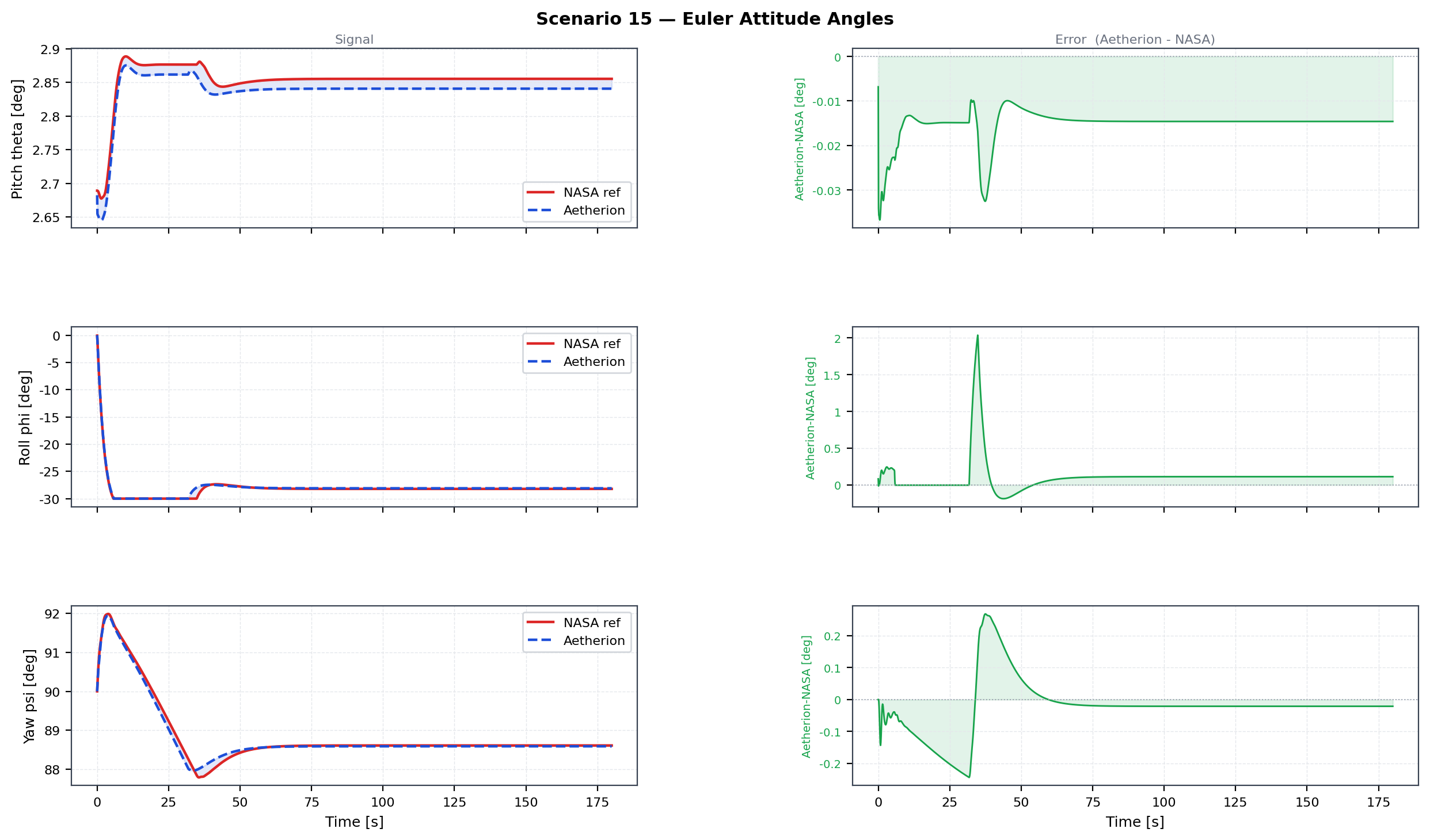
Scenario 15 Euler attitude angles — pitch, roll, yaw. The roll settles to ≈ −28° once the vehicle intercepts the circular track. Aetherion (blue dashed) vs NASA Atmos_15_sim_05 (red).
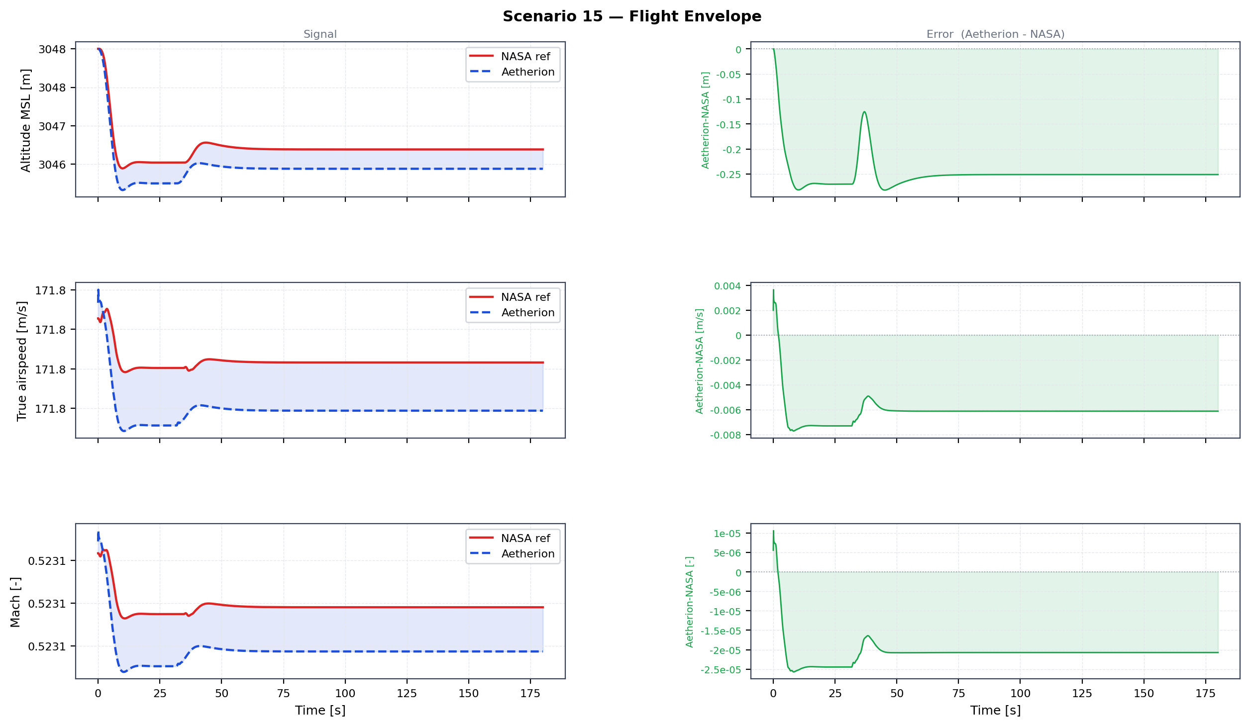
Scenario 15 flight envelope — altitude, TAS, Mach. Aetherion (blue dashed) vs NASA Atmos_15_sim_05 (red).
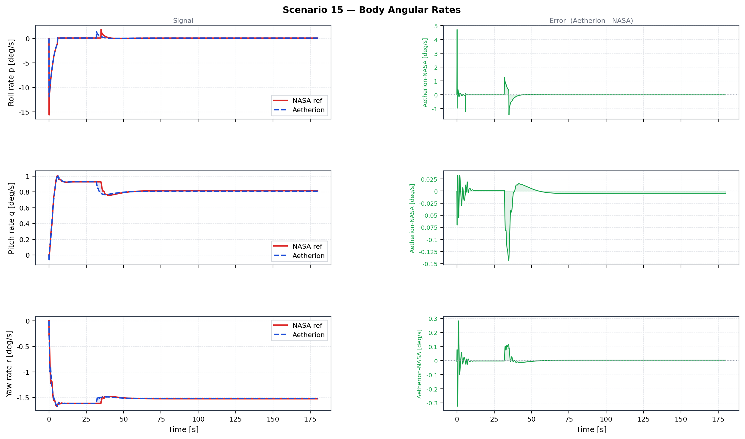
Scenario 15 body angular rates — roll, pitch, yaw rates. Aetherion (blue dashed) vs NASA Atmos_15_sim_05 (red).
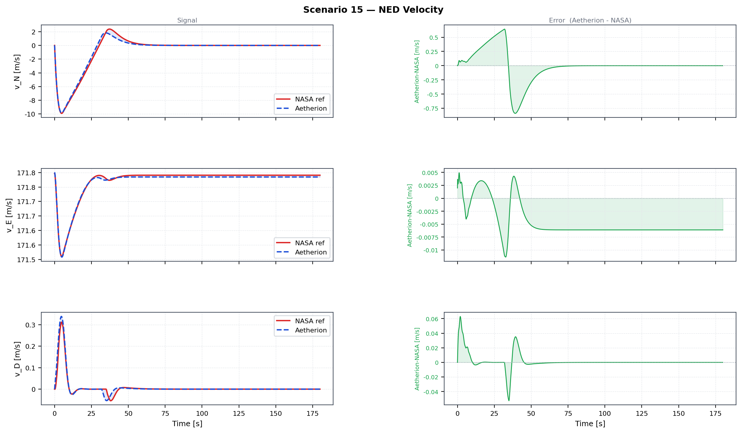
Scenario 15 NED velocity components — North, East, Down. Aetherion (blue dashed) vs NASA Atmos_15_sim_05 (red).
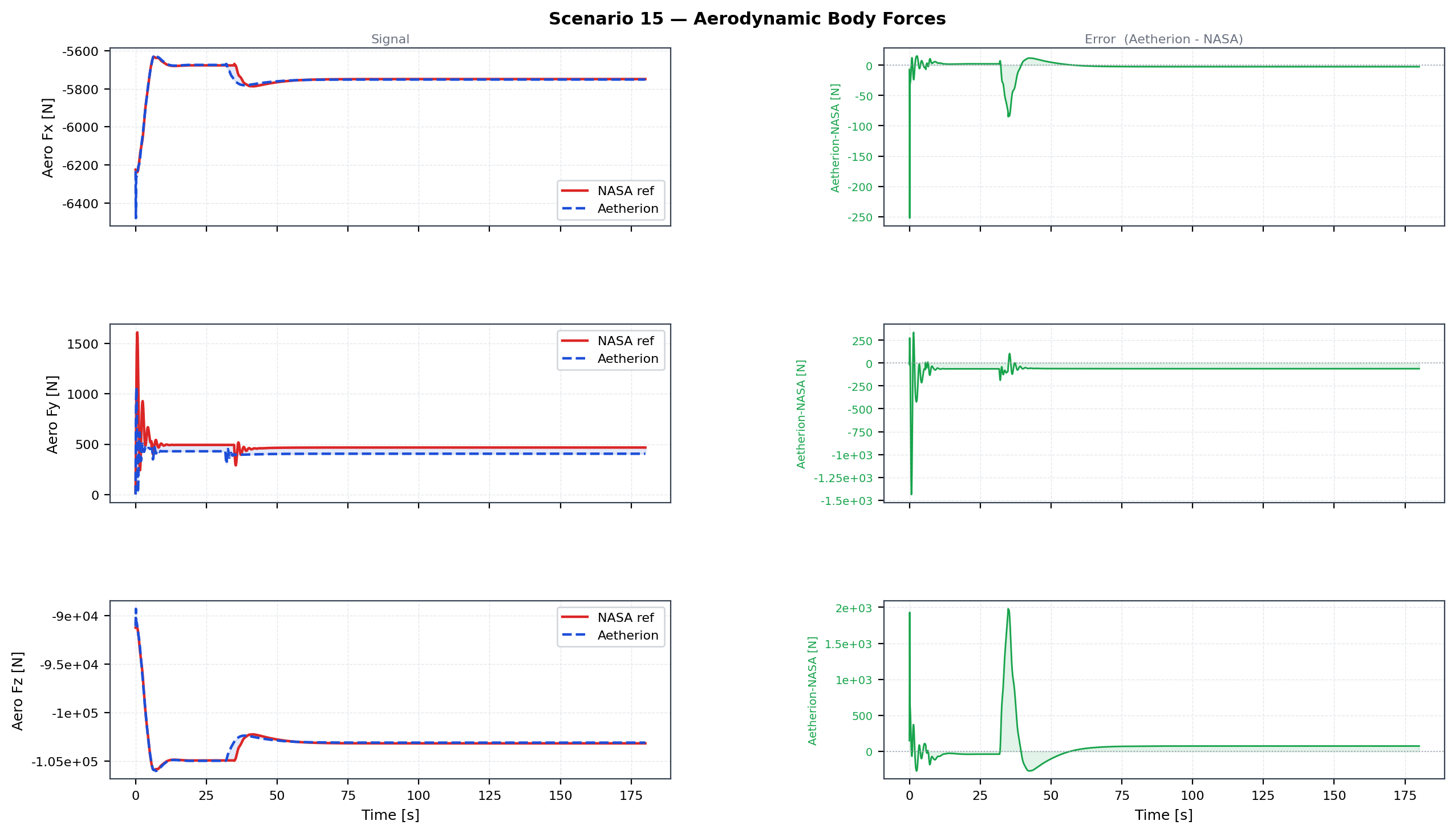
Scenario 15 aerodynamic body forces — X, Y, Z. Aetherion (blue dashed) vs NASA Atmos_15_sim_05 (red).
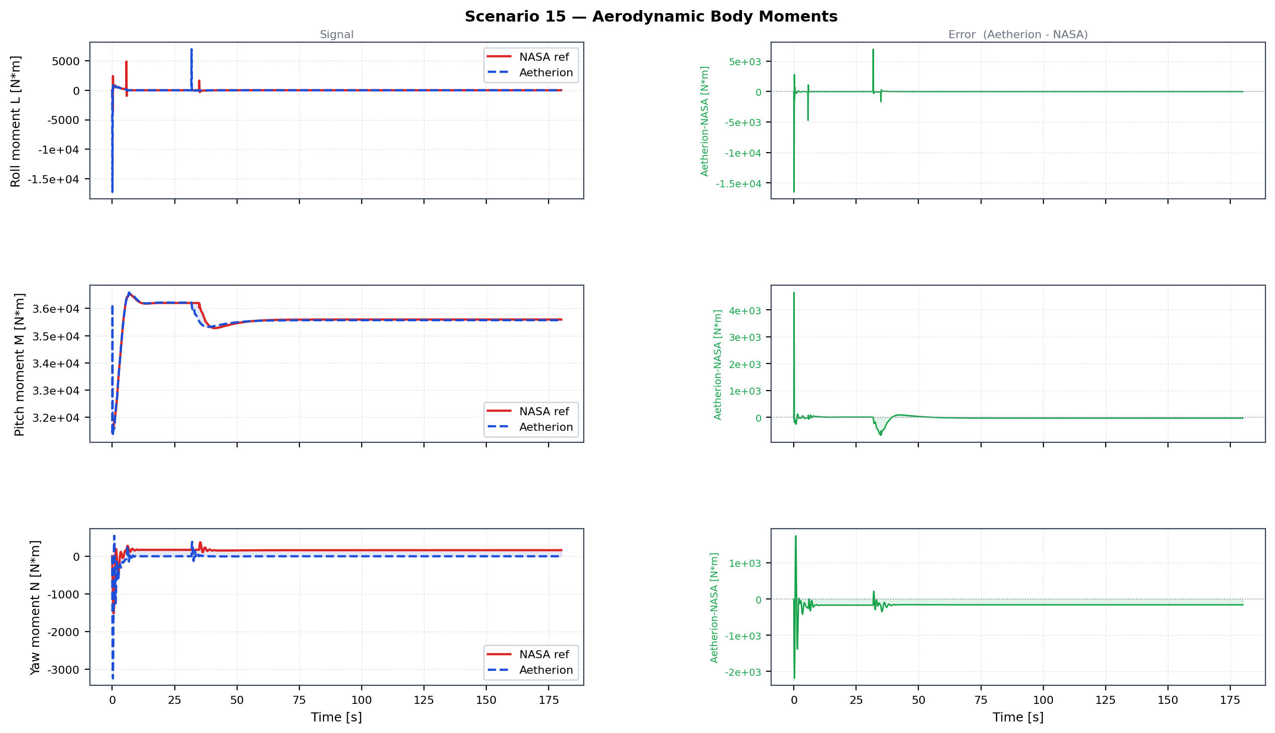
Scenario 15 aerodynamic body moments — L, M, N. Aetherion (blue dashed) vs NASA Atmos_15_sim_05 (red).
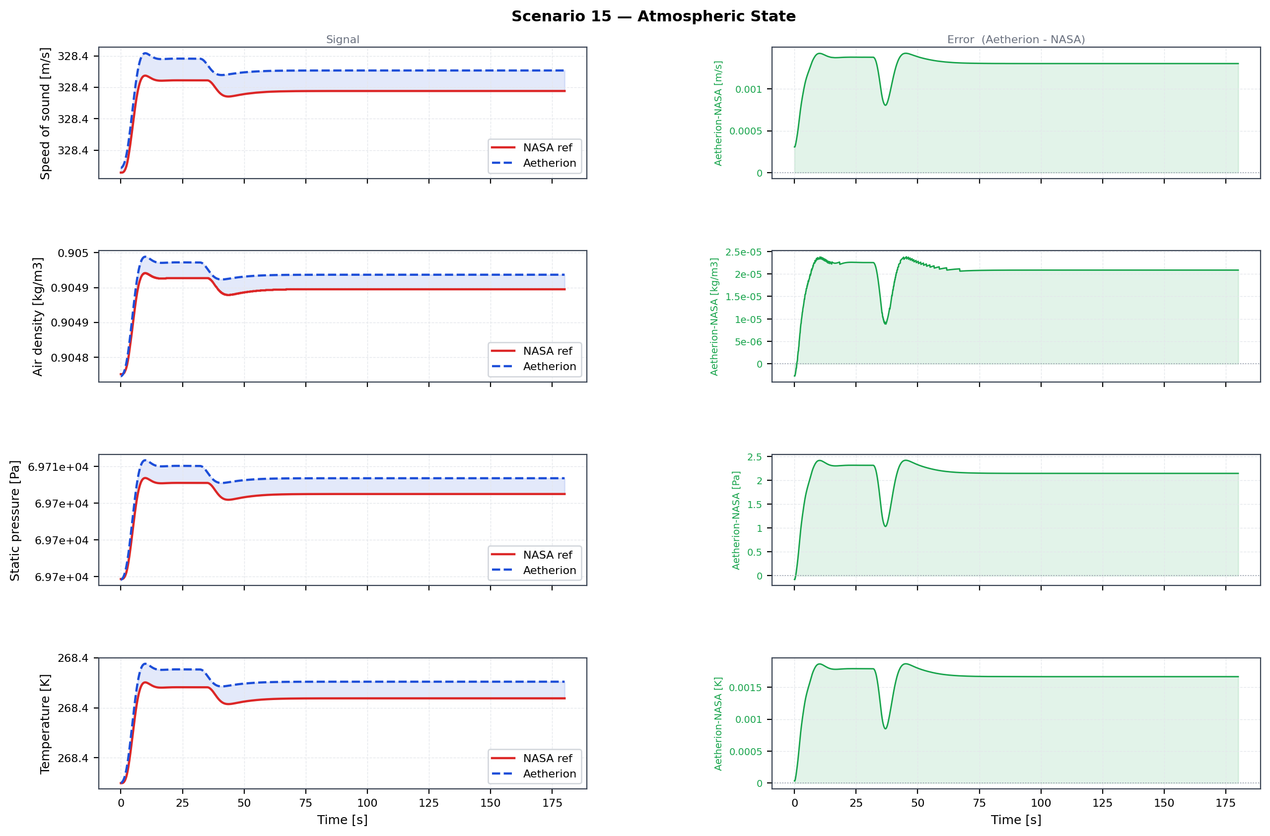
Scenario 15 atmosphere — temperature, density, pressure. Aetherion (blue dashed) vs NASA Atmos_15_sim_05 (red).
F-16 Equator/Date-Line Circumnavigation (NASA TM-2015-218675 Atmospheric Scenario 16)
Scenario overview
Scenario 16 complements Scenario 15 by exercising the equatorial edge case: a full six-DOF F-16 simulation that circumnavigates the intersection of the equator and the International Date Line (lat = 0°, lon = ±180°) on a 3-nautical-mile-radius circular track. The primary geodetic challenge is the date-line crossing — the vehicle’s geodetic longitude wraps across ±180° twice during the 180-second run, and the control system must handle the discontinuity without treating it as a large position error.
The control model is the same ``F16_gnc.dml`` used in Scenario 15.
Setting circlePoleSW to 0.0 activates the equator/IDL branch of
the circumnavigator: the DML model computes cross-track deviation from the
desired 3-nmi circle centred on the date-line/equator crossing and
commands the required bank angle to the heading autopilot, while altitude
and airspeed holds remain active throughout.
The vehicle is trimmed straight and level at 10 000 ft / 563.6 ft/s TAS (Mach 0.523) heading due north; the circumnavigating autopilot is engaged from the very first time step. Within approximately 30 s the aircraft has intercepted the circular track and settles into a steady left bank of ≈ 28°.
Circle geometry
The target circle is centred on the equator/date-line crossing point (lat = 0°, lon = ±180°). The DML measures cross-track deviation as a two-component Cartesian distance in a local flat-Earth frame centred on that point:
where
and \(\Delta\lambda = \lambda + 180°\) for \(\lambda < 0\), \(\Delta\lambda = \lambda - 180°\) for \(\lambda \geq 0\).
With \(R = 3\ \text{nmi}\) the circle circumference is:
At the trim TAS of 171.8 m/s the nominal circuit period is:
The 180-second run therefore covers approximately 319° of the full circle (the first ~30 s are spent intercepting the track from the initial heading-north condition; the remaining 150 s are at steady state).
The date line is crossed twice during the run: once between t = 30 s and t = 60 s (longitude jumps from ≈ −179.97° to ≈ +179.99°) and once between t = 150 s and t = 180 s (longitude returns from ≈ +179.99° to ≈ −179.97°).
Steady-state bank angle
For a coordinated level turn at radius \(R = 3\ \text{nmi} = 5\,556\ \text{m}\) and true airspeed \(V = 171.8\ \text{m/s}\):
The NASA reference CSV confirms roll ≈ −28.3° at steady state (t ≥ 60 s).
Circumnavigator GNC architecture
The equator/IDL branch of F16_gnc.dml computes:
degEFromTgt— piecewise longitude offset from the date line (\(\lambda + 180°\) if \(\lambda < 0\), else \(\lambda - 180°\)).ownshipN_ft,ownshipE_ft— flat-Earth North/East displacement from the circle centre in feet.latOffsetEquatorIDL— cross-track error \(\sqrt{N^2 + E^2} - R_\mathrm{circle}\).baseChiCmdEquatorIDL— tangential course command \(-\tfrac{180}{\pi}\operatorname{atan2}(N,E)\) (perpendicular to the radius vector, in the left-hand (CCW) sense).
These are selected by the circlePoleSW = 0.0 piecewise switch and fed
to the same heading/lateral autopilot used in Scenarios 13.1–15.
Initial and command conditions
Parameter |
Value |
|---|---|
Location |
0.000° N, 179.950° W (equator, just west of International Date Line) |
Altitude (initial & commanded) |
10 000 ft (3 048.0 m) |
Heading (initial) |
0° north |
TAS (trim) |
563.643 ft/s ≈ 333.95 kt (Mach 0.523) |
KEAS command |
computed from US1976 atmosphere at 10 000 ft |
Autopilot: |
0.0 (equator/IDL circumnavigator ON from t = 0) |
Geodesy / gravity |
WGS-84 rotating ellipsoid, J₂ gravity |
Atmosphere |
US Standard Atmosphere 1976, no wind |
Simulation duration |
180 s |
Trim result
The trim conditions at 10 000 ft / 563.643 ft/s TAS are identical to Scenarios 11 and 15 (same aircraft, same altitude):
Quantity |
Aetherion |
NASA ref |
|---|---|---|
α (trim) |
2.682° |
2.667° |
δe (trim) |
≈ −3.26° |
— |
Throttle (trim) |
≈ 13.9 % |
— |
Recommended run command
CircleEquatorDateLine --endTime 180 --timeStep 0.02 \
                      --outputFileName atmos_16_output.csv
The reference CSVs Atmos_16_sim_02/04/05.csv are copied to the build
directory post-build.
Validation results (NASA reference Atmos_16_sim_05)
The table below compares NASA and Aetherion trajectories at selected time steps. The vehicle intercepts the circular track by t ≈ 30 s and sustains steady-state circumnavigation for the remaining 150 s.
\(t\) [s] |
Alt [ft] |
Lat [°] |
Lon [°] |
Yaw [°] |
Pitch [°] |
Roll [°] |
Mach |
|---|---|---|---|---|---|---|---|
0 |
10 000.00 |
0.0000 |
−179.950 |
0.00 |
2.665 |
0.000 |
0.5231 |
30 |
9 994.56 |
+0.0408 |
−179.968 |
−53.73 |
2.847 |
−29.996 |
0.5231 |
60 |
9 995.25 |
+0.0497 |
+179.988 |
−105.36 |
2.825 |
−27.785 |
0.5231 |
90 |
9 995.19 |
+0.0209 |
+179.953 |
−157.08 |
2.825 |
−28.316 |
0.5231 |
120 |
9 995.33 |
−0.0240 |
+179.955 |
+150.53 |
2.818 |
−28.449 |
0.5231 |
150 |
9 995.55 |
−0.0504 |
+179.991 |
+98.59 |
2.809 |
−28.126 |
0.5231 |
180 |
9 995.50 |
−0.0382 |
−179.966 |
+47.03 |
2.811 |
−28.206 |
0.5231 |
Key observations from the reference trajectory:
Altitude holds within 6 ft of the commanded 10 000 ft after the initial transient.
Bank angle stabilises at −28.3° (left bank) from t ≈ 60 s onward, consistent with the analytical prediction of −28.3° for a 3-nmi radius turn.
Date-line crossings — longitude wraps from ≈ −180° to ≈ +180° between t = 30 s and t = 60 s, and from ≈ +180° to ≈ −180° between t = 150 s and t = 180 s, with no discontinuity in the physical trajectory.
Yaw wraps through ±180° (from −157° at t = 90 s to +151° at t = 120 s), confirming correct heading-angle wrapping.
Latitude oscillates between ≈ +0.05° and ≈ −0.05°, i.e., the orbit straddles the equator symmetrically.
Aetherion simulation results
\(t\) [s] |
Alt [ft] |
Lat [°] |
Lon [°] |
Yaw [°] |
Pitch [°] |
Roll [°] |
Mach |
|---|---|---|---|---|---|---|---|
0 |
10 000.00 |
0.0000 |
−179.950 |
0.00 |
2.665 |
0.000 |
0.5231 |
30 |
9 994.55 |
+0.0408 |
−179.968 |
−53.69 |
2.848 |
−29.995 |
0.5231 |
60 |
9 995.24 |
+0.0497 |
+179.988 |
−105.35 |
2.825 |
−27.785 |
0.5231 |
90 |
9 995.17 |
+0.0209 |
+179.953 |
−157.06 |
2.826 |
−28.337 |
0.5231 |
120 |
9 995.32 |
−0.0240 |
+179.955 |
+150.55 |
2.819 |
−28.471 |
0.5231 |
150 |
9 995.54 |
−0.0504 |
+179.991 |
+98.62 |
2.810 |
−28.147 |
0.5231 |
180 |
9 995.49 |
−0.0382 |
−179.966 |
+47.05 |
2.812 |
−28.227 |
0.5231 |
Against simulation 05 the maximum latitude error is 0.000019° (2 m) and the maximum longitude error 0.0000° over the whole trajectory; altitude agrees to 0.12 ft. Roll agrees to 0.02° from t = 60 s onward (0.8° peak while the circle is being captured), and altitude is held within 5.5 ft of 10 000 ft from t = 30 s onward.
Validation figures
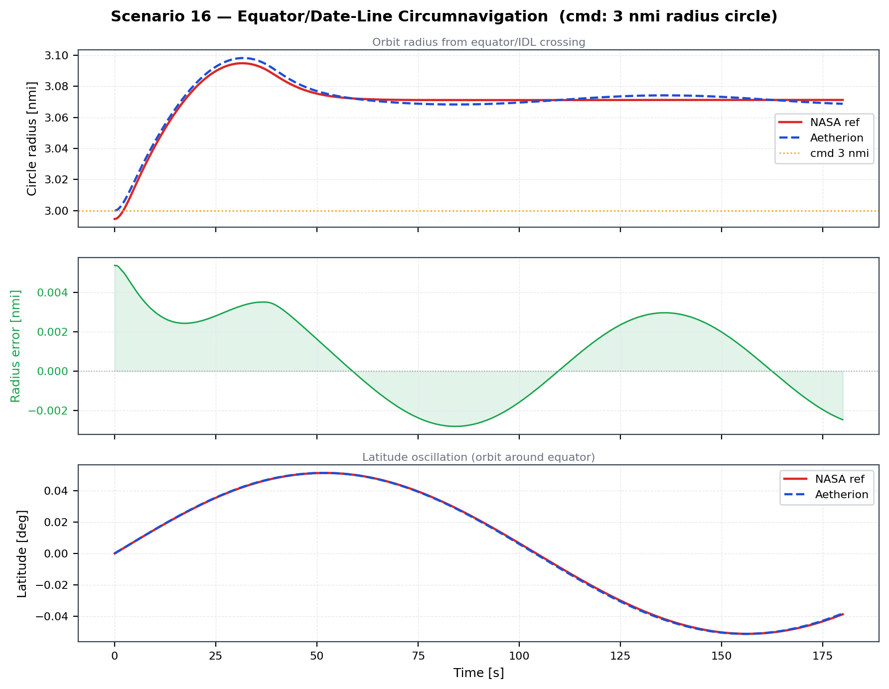
Scenario 16 orbit radius from the equator/IDL crossing (top) and latitude oscillation (bottom). The circumnavigator holds the aircraft within < 0.01 nmi of the commanded 3-nmi circle from t ≈ 30 s onward, and the orbit straddles the equator symmetrically. Aetherion (blue dashed) vs NASA Atmos_16_sim_05 (red).
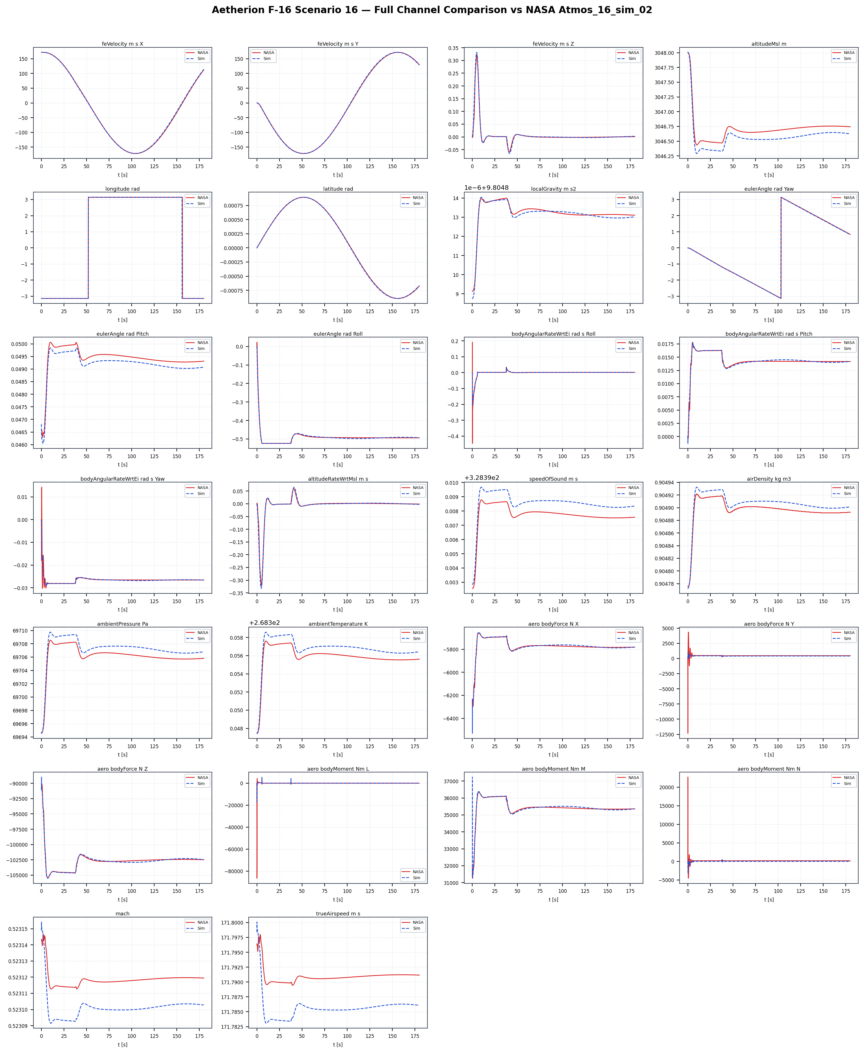
Scenario 16 simulation overview — 180 s equator/date-line circumnavigation. Aetherion (blue dashed) vs NASA Atmos_16_sim_05 (red).
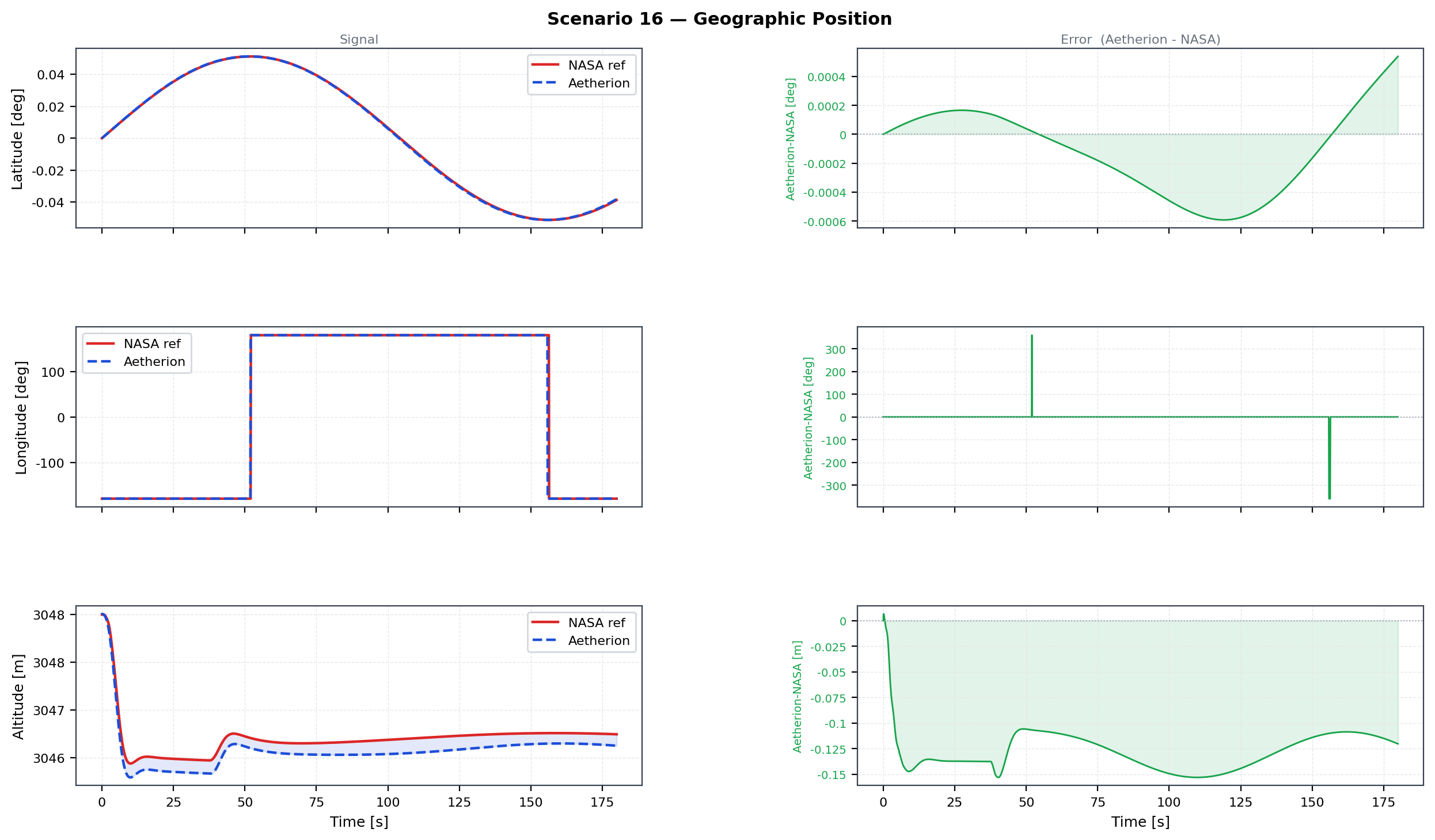
Scenario 16 geodetic position — altitude, latitude, and longitude (note the two date-line crossings near t = 45 s and t = 165 s). Aetherion (blue dashed) vs NASA Atmos_16_sim_05 (red).
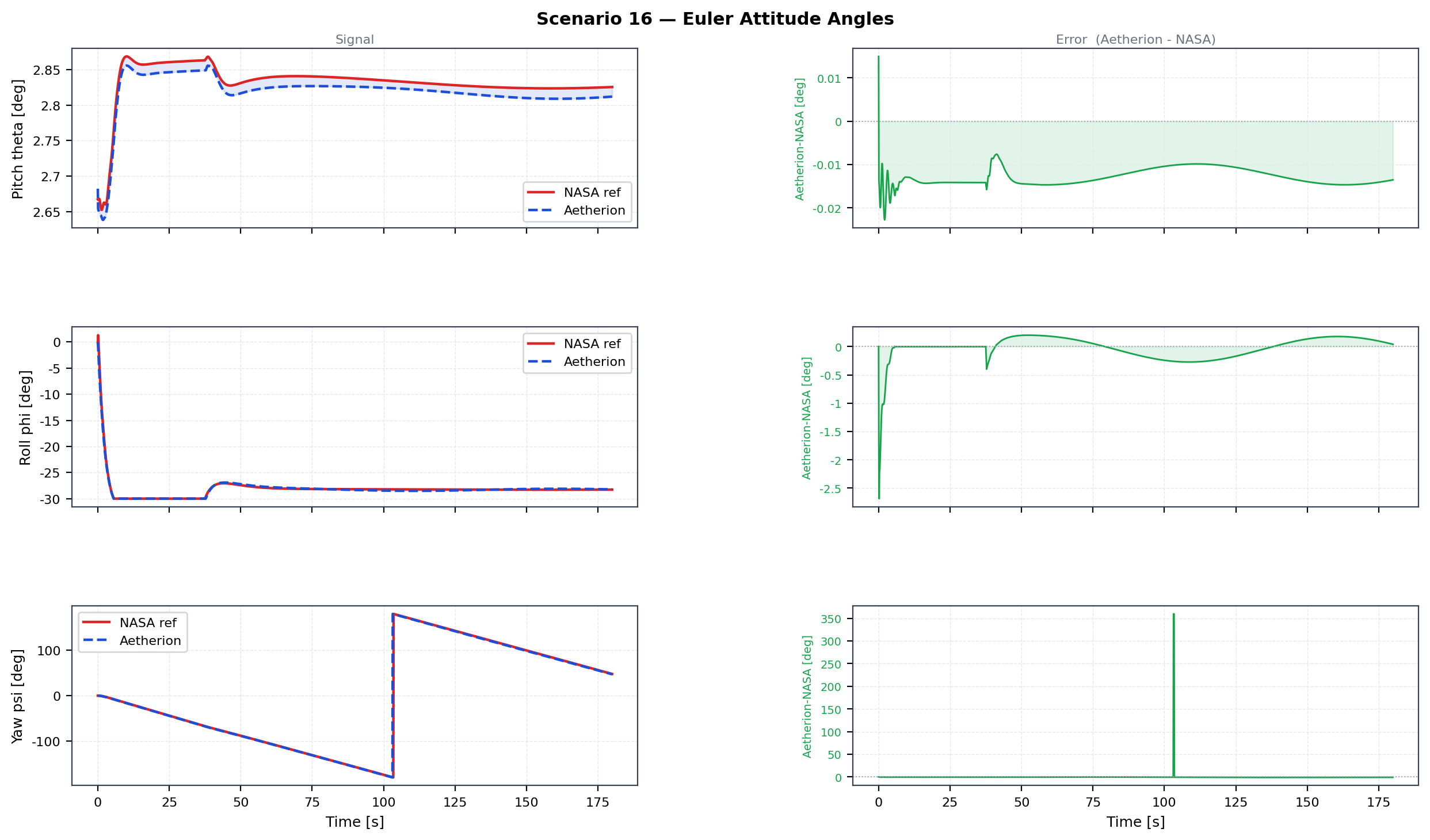
Scenario 16 Euler attitude angles — pitch, roll, yaw. The roll settles to ≈ −28° once the vehicle intercepts the circular track; the yaw wraps through ±180° during the orbit. Aetherion (blue dashed) vs NASA Atmos_16_sim_05 (red).
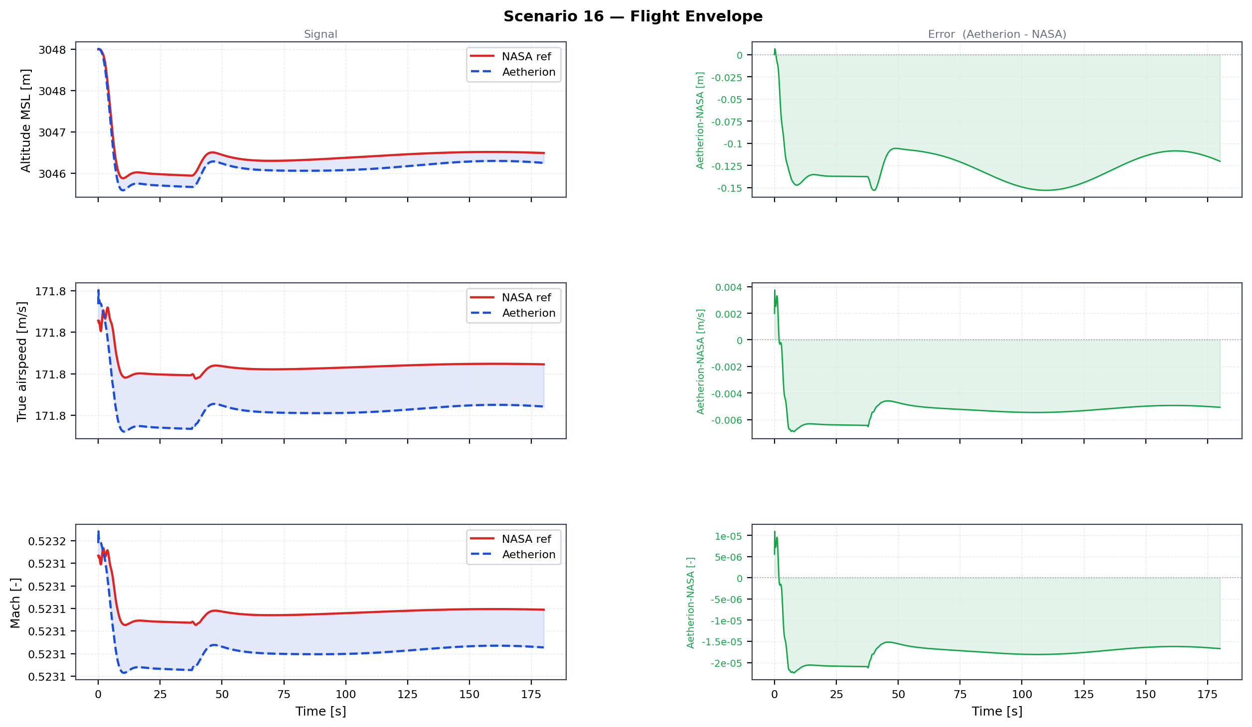
Scenario 16 flight envelope — altitude, TAS, Mach. Aetherion (blue dashed) vs NASA Atmos_16_sim_05 (red).
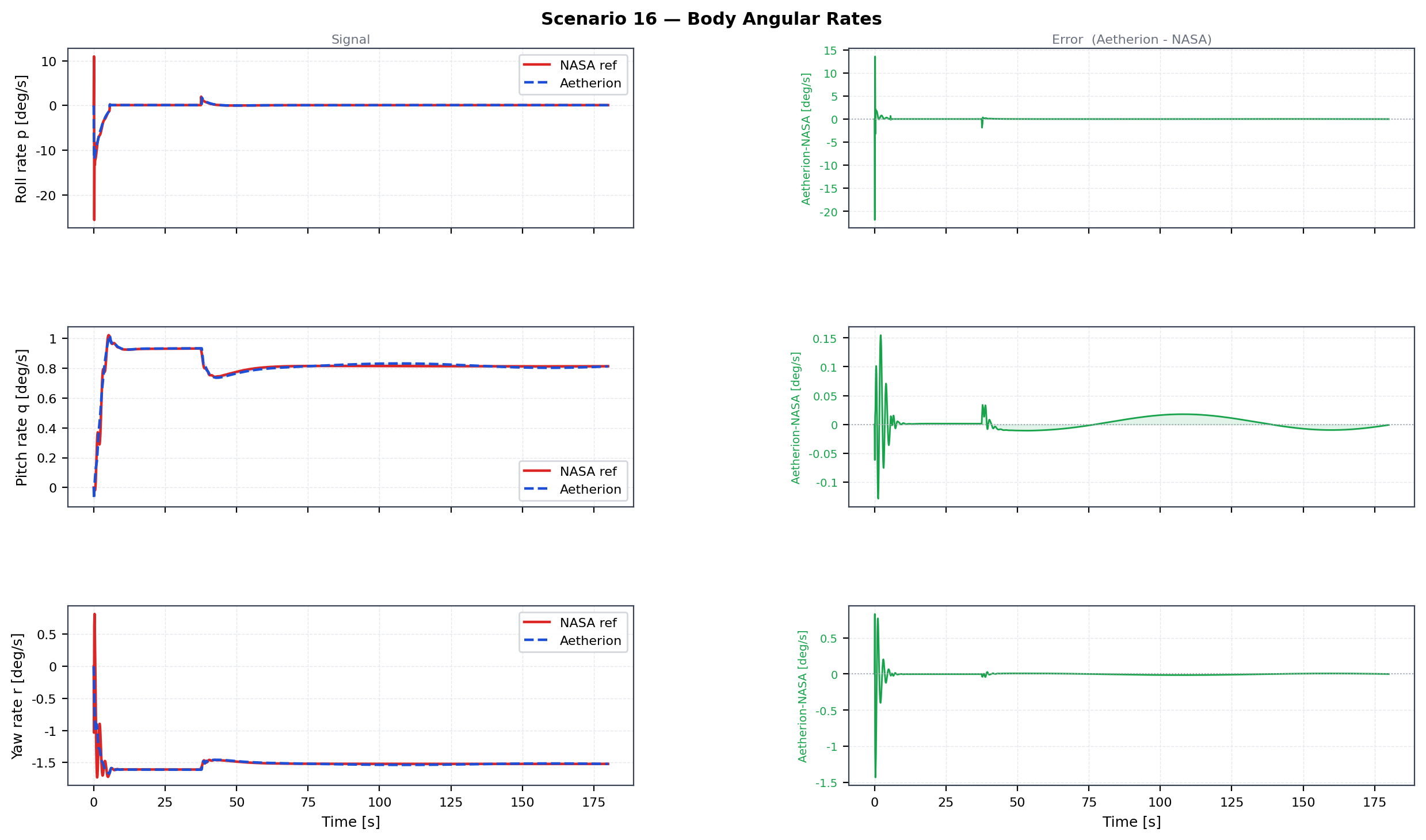
Scenario 16 body angular rates — roll, pitch, yaw rates. Aetherion (blue dashed) vs NASA Atmos_16_sim_05 (red).
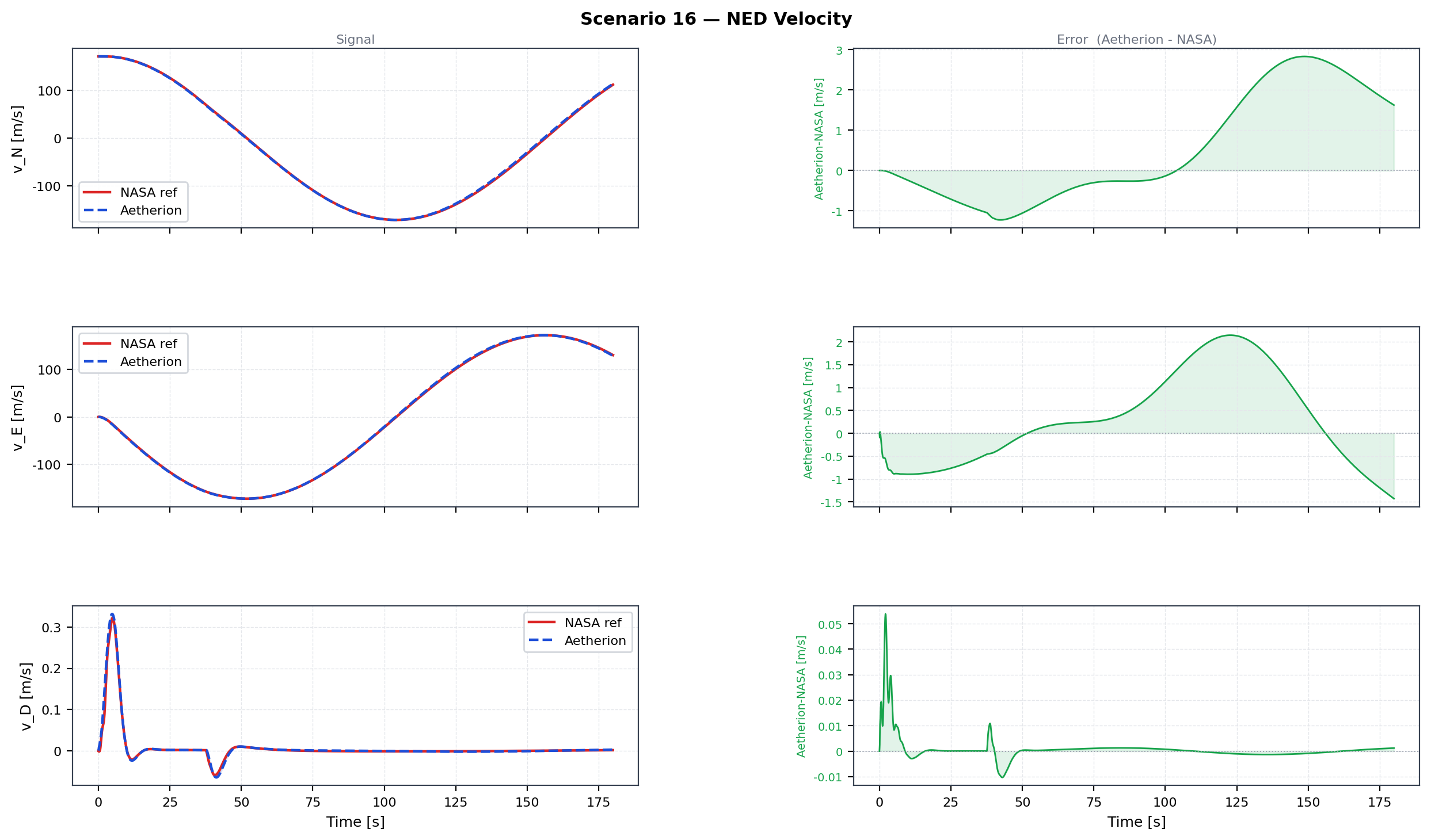
Scenario 16 NED velocity components — North, East, Down. Aetherion (blue dashed) vs NASA Atmos_16_sim_05 (red).
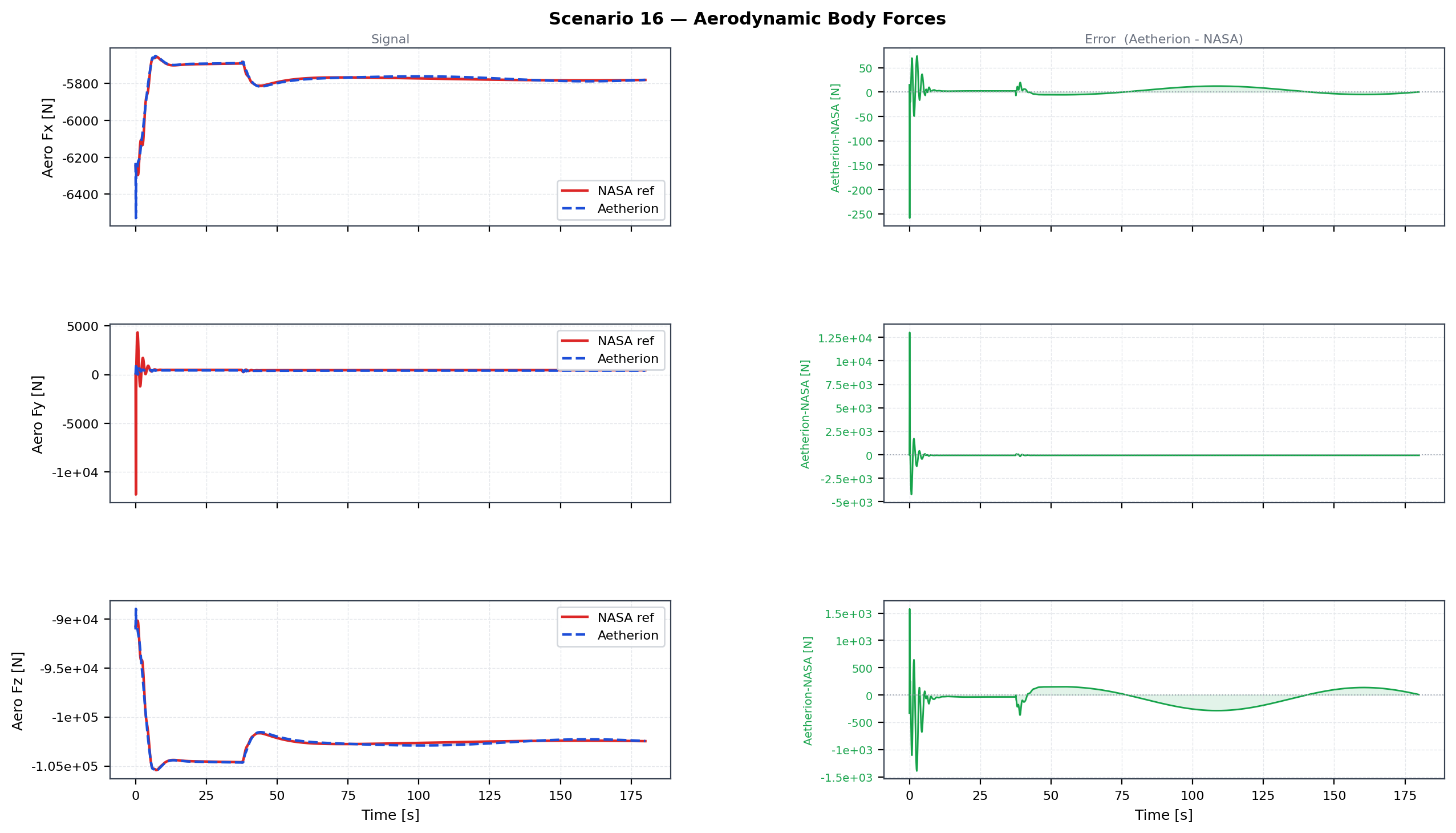
Scenario 16 aerodynamic body forces — X, Y, Z. Aetherion (blue dashed) vs NASA Atmos_16_sim_05 (red).
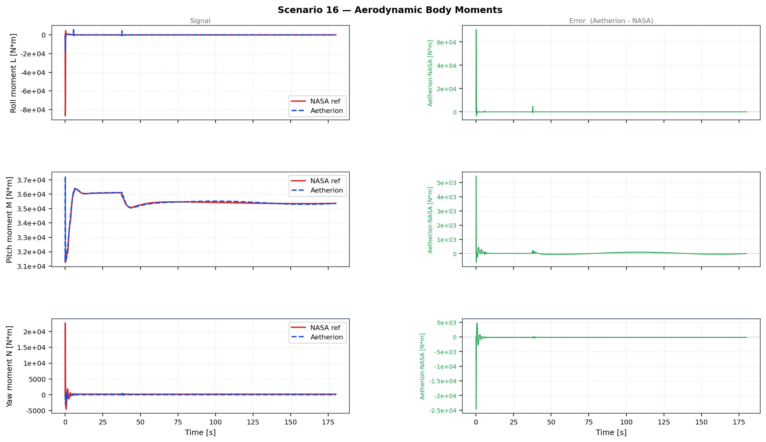
Scenario 16 aerodynamic body moments — L, M, N. Aetherion (blue dashed) vs NASA Atmos_16_sim_05 (red).
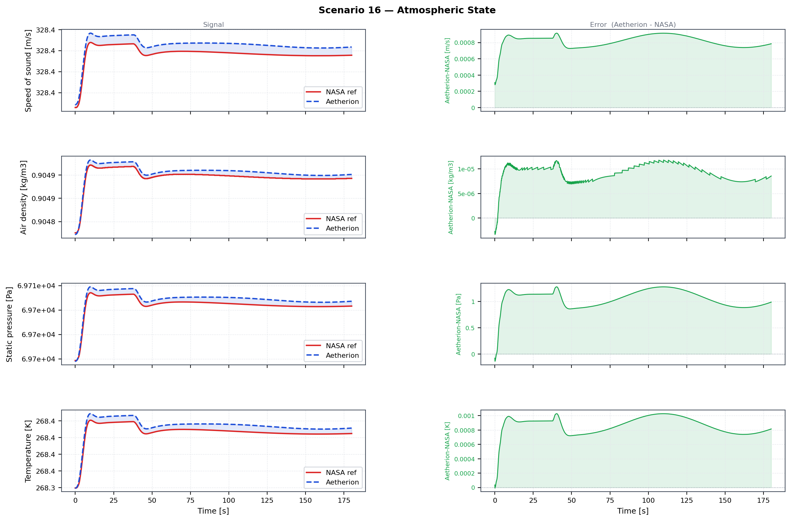
Scenario 16 atmosphere — temperature, density, pressure. Aetherion (blue dashed) vs NASA Atmos_16_sim_05 (red).
Two-Stage Rocket to Orbit (NASA TM-2015-218675 Atmospheric Scenario 17)
Reference: NASA TM-2015-218675, Atmospheric and Space Flight Vehicle Equations of Motion, Appendix B, Section B.1.17 — Atmospheric Simulation 17.
DAVE-ML data files: data/TwoStageRocket_S119_source/twostage_aero.dml,
twostage_inertia.dml, twostage_prop.dml
(authored by E. M. Queen and B. Jackson, NASA Langley Research Center, 2013).
Scenario Overview
This is the most complex atmospheric example in the NASA reference: a full six-degree-of-freedom simulation of an open-loop two-stage rocket ascending to orbit from the equatorial prime meridian. Unlike the F-16 scenarios, the vehicle is not trimmed — it follows a gravity-turn trajectory dictated entirely by its initial attitude and the physical forces acting on it.
Three new phenomena distinguish this example from all earlier scenarios:
Variable mass — propellant is consumed continuously, shrinking the total mass and shifting the centre of gravity (CG) along the body axis.
Stage separation — when Stage 1 propellant is exhausted the first-stage hardware (35 000 kg) is jettisoned instantaneously; Stage 2 ignites immediately.
CG–MRC offset — the DAVE-ML aerodynamic and inertia models define moments about a fixed Moment Reference Centre (MRC) while gravity and inertia forces act at the (moving) CG; the equations of motion must correct for this offset.
The vehicle is based on Eric Queen’s conceptual two-stage-to-orbit design (source document: twostagetoorbit.pptx, NASA LaRC, 2013).
Physics Model
The simulation composes four physics policies into a single VectorField:
using TwoStageRocketVF = RigidBody::VectorField<
    RocketGravityPolicy,              // J₂ gravity + CG–MRC moment transfer
    RocketAeroPolicy,                 // DAVE-ML CL/CD/CY/Cm/Cn, wind-to-body
    FlightDynamics::AxialThrustPolicy,// body +x thrust from propulsion DML
    FlightDynamics::LinearBurnPolicy  // variable mdot, updated each step (ZOH)
>;

using Stepper = RigidBody::SixDoFStepper<TwoStageRocketVF>;
All four policies are evaluated at every stage evaluation of the Radau IIA RKMK integrator. The mass properties (inertia matrix, CG offset) and propulsion state (thrust, mass flow rate) are refreshed once per integration step using a zero-order-hold (ZOH) scheme.
Inertia Model — twostage_inertia.dml
The inertia model computes five outputs as piecewise-linear functions of the cumulative fuel consumed in each stage and a binary staging flag.
Inputs
Variable ID |
Unit |
Description |
|---|---|---|
|
— |
0 = Stage 1 active; > 0 = Stage 2 active (S1 jettisoned) |
|
kg |
Cumulative Stage-1 propellant consumed |
|
kg |
Cumulative Stage-2 propellant consumed |
Reference constants
Quantity |
Stage 1 (ignition) |
Stage 1 (burnout) |
Notes |
|---|---|---|---|
Mass \(m\) [kg] |
314 000 |
134 000 |
Fuel capacity: 180 000 kg |
\(x_{CG}\) [m aft of nose] |
16.919 |
9.422 |
CG travels 7.50 m forward as S1 burns |
\(I_{xx}\) [kg·m²] |
353 250 |
150 750 |
Roll (axial) inertia |
\(I_{yy} = I_{zz}\) [kg·m²] |
33 501 637 |
10 886 637 |
Pitch / yaw inertia (axisymmetric) |
MRC position [m aft of nose] |
16.919 |
16.919 |
Fixed during Stage 1 |
Quantity |
Stage 2 (ignition) |
Stage 2 (burnout) |
Notes |
|---|---|---|---|
Mass \(m\) [kg] |
99 000 |
19 000 |
Fuel capacity: 80 000 kg |
\(x_{CG}\) [m aft of nose] |
4.798 |
3.947 |
CG travels 0.85 m forward as S2 burns |
\(I_{xx}\) [kg·m²] |
111 375 |
21 375 |
Roll inertia (S2 only) |
\(I_{yy} = I_{zz}\) [kg·m²] |
941 064 |
212 385 |
Pitch / yaw inertia (S2 only) |
MRC position [m aft of nose] |
4.798 |
4.798 |
Fixed during Stage 2 |
Fuel fraction and linear interpolation
The DML first computes a remaining fuel fraction for each stage:
where \(C_1 = 180\,000\ \text{kg}\) and \(C_2 = 80\,000\ \text{kg}\) are the propellant capacities. \(f_i = 1\) when the stage is full; \(f_i = 0\) at burnout.
Every mass property \(P\) is then linearly interpolated between its ignition value \(P_{\text{ign}}\) and its burnout value \(P_{\text{bo}}\):
This single formula covers mass, \(x_{CG}\), \(I_{xx}\),
\(I_{yy}\), and \(I_{zz}\). The active stage is selected by the
piecewise condition on stagedFlag:
CG–MRC offset (DXCG)
The aerodynamic lookup tables define moments about the Moment Reference Centre (MRC). Because the CG shifts as propellant is consumed, the DML tracks the signed offset:
During Stage 1, the MRC is fixed at 16.919 m aft of the nose. As propellant burns, \(x_{CG}\) decreases (moves forward), so DXCG grows from 0 m (at liftoff, where CG ≅ MRC) to +7.50 m at S1 burnout. During Stage 2 the MRC shifts to 4.798 m aft of the nose.
All products of inertia (\(I_{xz}\), \(I_{xy}\), \(I_{yz}\)) are identically zero — the vehicle is axisymmetric.
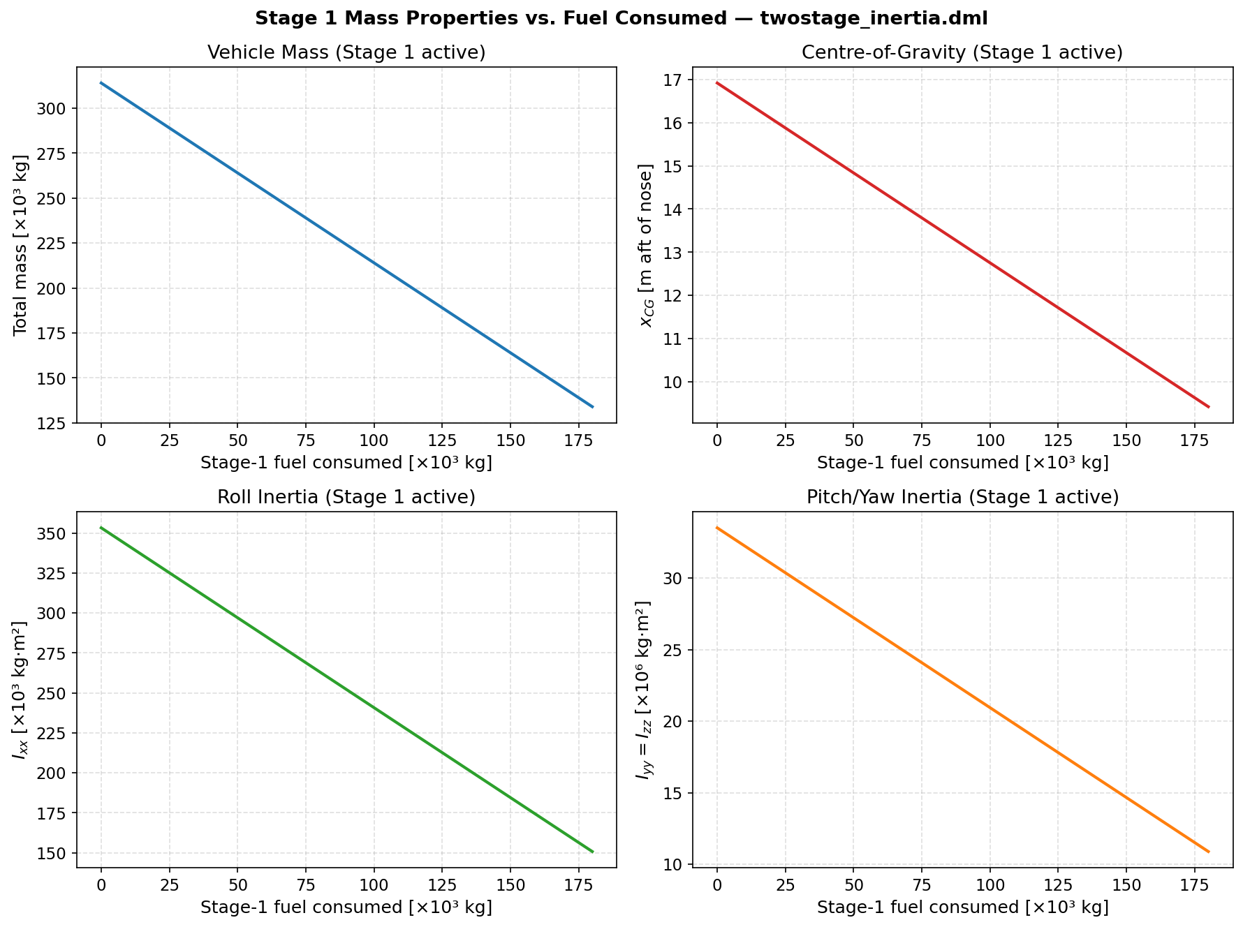
Stage 1 mass, CG position, roll inertia \(I_{xx}\), and pitch/yaw inertia \(I_{yy}\) as functions of cumulative fuel consumed. All quantities vary linearly with fuel fraction \(f_1\).
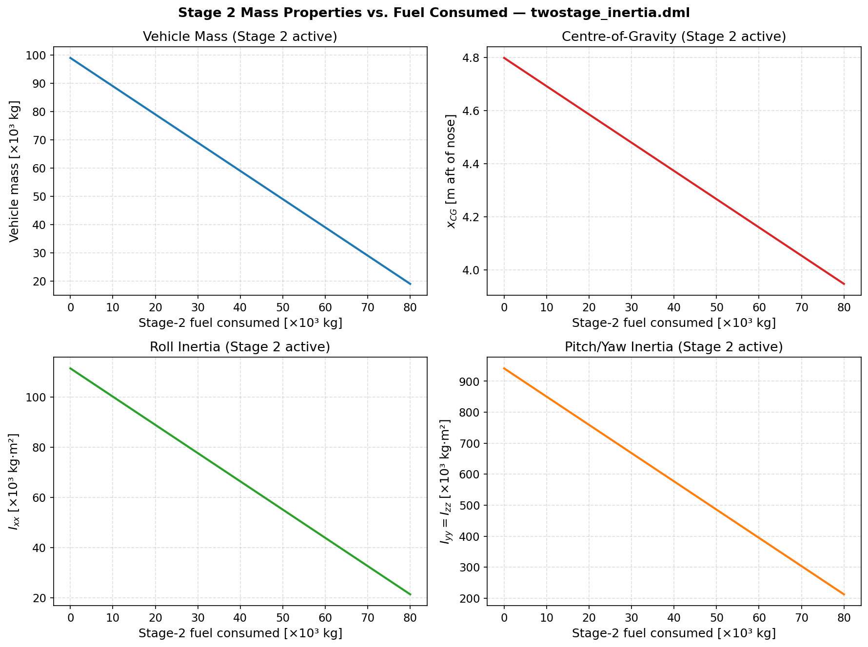
Stage 2 mass properties after separation. The much smaller inertias (note the axis scales) reflect the slender upper-stage geometry.
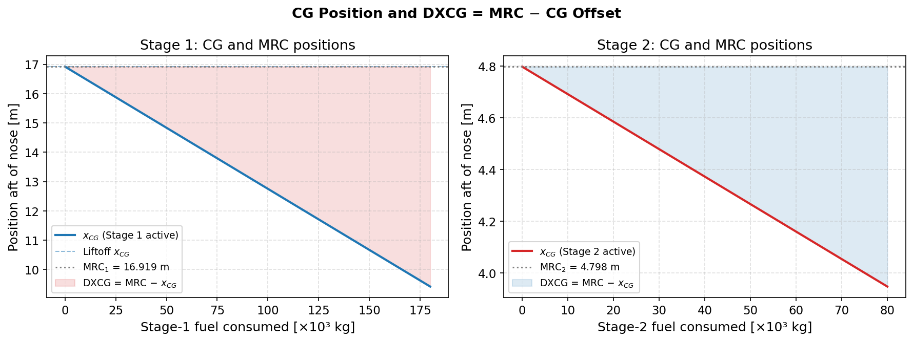
CG position (solid line) and fixed MRC (dashed) for each stage. The shaded band is the DXCG offset that enters the gravity moment-transfer correction. At Stage 1 liftoff the CG and MRC nearly coincide (DXCG ≈ 0); by burnout DXCG has grown to ~7.5 m, creating a substantial gravity moment.
Propulsion Model — twostage_prop.dml
Inputs
Variable ID |
Unit |
Description |
|---|---|---|
|
— |
> 0 when Stage 1 is burning |
|
— |
> 0 when Stage 2 is burning |
Engine constants
Quantity |
Stage 1 |
Stage 2 |
Notes |
|---|---|---|---|
Maximum thrust \(T\) [N] |
17 000 000 |
5 000 000 |
Constant during burn (no throttle model) |
Specific impulse \(I_{sp}\) [s] |
360 |
390 |
S2 is more efficient (higher-altitude vacuum Isp) |
Thrust (piecewise constant)
Thrust acts solely along the body \(+x\) axis (nose direction); lateral and axial moment components from thrust are identically zero:
Propellant mass flow rate (Tsiolkovsky)
The propellant consumption rate follows directly from the rocket equation definition of specific impulse:
Numerically:
Stage |
\(T\) [N] |
\(I_{sp}\) [s] |
\(\dot{m}\) [kg/s] |
|---|---|---|---|
1 |
17 000 000 |
360 |
\(\approx 4\,810.5\) |
2 |
5 000 000 |
390 |
\(\approx 1\,307.3\) |
At these rates, Stage 1 exhausts its 180 000 kg propellant in \(180\,000 / 4810.5 \approx 37.4\ \text{s}\), and Stage 2 exhausts its 80 000 kg in \(80\,000 / 1307.3 \approx 61.2\ \text{s}\).
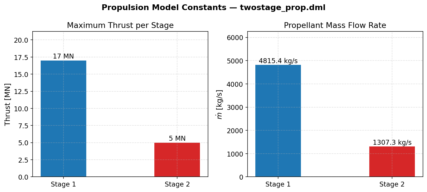
Maximum thrust and derived propellant mass flow rate for each stage. Stage 1 produces 3.4× more thrust and burns propellant 3.7× faster than Stage 2; Stage 2 compensates with a 8.3% higher specific impulse.
Staging event
When RocketStageModel::advance() detects that the cumulative
Stage-1 fuel consumed equals the capacity \(C_1 = 180\,000\ \text{kg}\),
it sets the staging flag and returns true. The simulator then applies
a discrete mass drop of \(\Delta m = 35\,000\ \text{kg}\) to the ODE
state, representing the jettison of the empty Stage-1 hardware:
The MRC immediately shifts from 16.919 m (S1 reference) to 4.798 m (S2 reference) and the spatial inertia matrix is rebuilt for the S2-only configuration.
Aerodynamic Model — twostage_aero.dml
The aerodynamic model receives two scalar inputs — angle of attack \(\alpha\) and sideslip angle \(\beta\) (both in degrees) — and returns five force/moment coefficients. All moments are defined about the current MRC.
Reference geometry
Quantity (DAVE-ML ID) |
Value |
Description |
|---|---|---|
Reference area \(S_{\text{ref}}\) ( |
7.0 m² |
Approximate frontal area of the rocket base |
Longitudinal ref. length \(\bar{c}\) ( |
3.0 m |
Used to non-dimensionalise pitching moment |
Lateral ref. length \(b\) ( |
3.0 m |
Used to non-dimensionalise yawing moment |
Total angle of attack
Before the drag table lookup the DML computes a total angle of attack that combines both the pitch and sideslip contributions:
This makes \(C_D\) symmetric with respect to the direction of incidence rather than purely pitch-plane.
Lookup tables and breakpoints
Force coefficients — 11-point tables, extrapolation clamped to ±10°:
α (β) [°] |
−10 |
−8 |
−6 |
−4 |
−2 |
0 |
+2 |
+4 |
+6 |
+8 |
+10 |
|---|---|---|---|---|---|---|---|---|---|---|---|
\(C_L(\alpha)\) |
−1.60 |
−1.00 |
−0.73 |
−0.49 |
−0.24 |
0 |
+0.24 |
+0.49 |
+0.73 |
+1.00 |
+1.60 |
\(C_D(\alpha_T)\) |
0.48 |
0.38 |
0.31 |
0.25 |
0.23 |
0.21 |
0.23 |
0.25 |
0.31 |
0.38 |
0.48 |
\(C_Y(\beta)\) |
+1.60 |
+1.00 |
+0.73 |
+0.49 |
+0.24 |
0 |
−0.24 |
−0.49 |
−0.73 |
−1.00 |
−1.60 |
Observations: \(C_L(\alpha)\) and \(C_Y(\beta)\) are odd functions (antisymmetric); \(C_D(\alpha_T)\) is an even function with a minimum value of 0.21 at zero incidence, rising to 0.48 at ±10°.
Moment coefficients — 3-point linear tables, range ±20°:
Coefficient |
α (β) = −20° |
0° |
+20° |
Slope |
|---|---|---|---|---|
\(C_m(\alpha)\) |
+0.60 |
0 |
−0.60 |
−0.03 / deg |
\(C_n(\beta)\) |
−0.60 |
0 |
+0.60 |
+0.03 / deg |
Both moment tables are linear and pass through zero at zero incidence. \(C_m\) is statically stable in pitch (negative slope → restoring moment for positive \(\alpha\)); \(C_n\) is statically stable in yaw. The rolling moment coefficient is identically zero (axisymmetric vehicle).
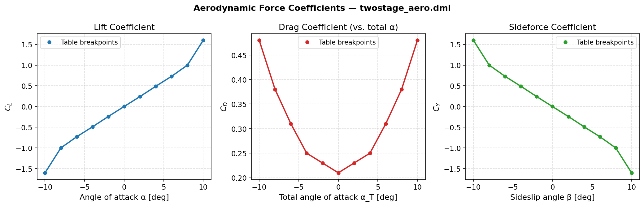
Lift (\(C_L\)), drag (\(C_D\)), and sideforce (\(C_Y\)) coefficients from the DAVE-ML lookup tables. Filled circles mark the 11 breakpoint values; the solid lines are the piecewise-linear interpolant used by the simulator. \(C_D\) uses the total angle of attack \(\alpha_T = \sqrt{\alpha^2+\beta^2}\) as its independent variable.
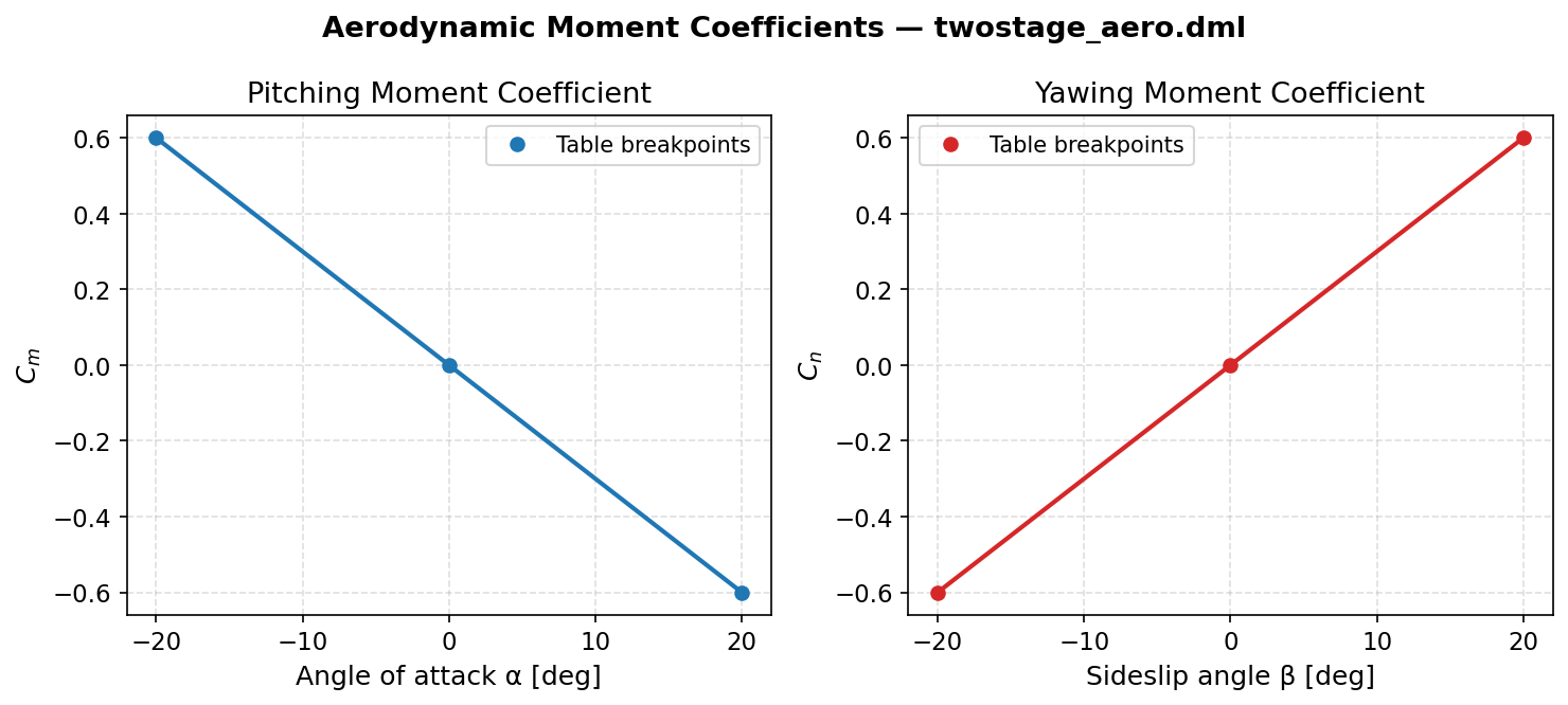
Pitching (\(C_m\)) and yawing (\(C_n\)) moment coefficients. The 3-breakpoint linear tables give a constant slope of ±0.03 /deg, reflecting a simple static stability model. \(C_l = 0\) (axisymmetric).
Dynamic pressure
The atmosphere-relative airspeed and dynamic pressure are computed at each integrator stage evaluation:
where \(\mathbf{r}\) is the ECI position vector, \(\boldsymbol{\omega}_E = [0,\,0,\,\omega_E]^\top\) in ECI with \(\omega_E = 7.292\,115 \times 10^{-5}\ \text{rad/s}\), and \(R_{BI}\) rotates ECI to body frame. The atmosphere-relative speed is:
and the dynamic pressure:
where \(\rho(h)\) is the US Standard Atmosphere 1976 density at the current geocentric altitude \(h \approx \lVert\mathbf{r}\rVert - R_e\).
Aerodynamic angles
From the atmosphere-relative velocity components \((u, v, w)\) in the body frame:
Both angles are passed to the DAVE-ML model in degrees. Table lookups are clamped at ±10° for force coefficients and ±20° for moment coefficients (no extrapolation).
Wind-to-body force transform
Force coefficients are defined in the wind frame \(\mathbf{F}_w = [-C_D,\;C_Y,\;-C_L]^\top \bar{q}S\) (drag opposing motion, lift perpendicular to drag, sideforce positive starboard). The wind-to-body rotation matrix is:
Expanding \(\mathbf{F}_B = R_{BW}\,\mathbf{F}_w\) with \(c_\alpha = \cos\alpha\), \(s_\alpha = \sin\alpha\), \(c_\beta = \cos\beta\), \(s_\beta = \sin\beta\):
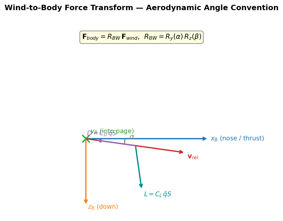
Sign convention for aerodynamic angle of attack \(\alpha\) and the wind-to-body force transform. Drag \(D\) opposes the velocity vector; lift \(L\) is perpendicular (upward in the body \(-z\) direction for positive \(\alpha\)). The moment axis \(y_B\) points into the page.
Aerodynamic moments (about MRC)
The DML moment outputs are already defined about the MRC so no transfer correction is required here:
Gravity Policy — J₂ with CG–MRC Moment Transfer
The simulator integrates the Newton–Euler equations about the MRC, but gravity acts at the CG. When these two points do not coincide, gravity produces an additional moment.
The gravitational acceleration in the ECI frame uses the J₂ zonal harmonic:
where \(\mu = 3.986\,004\,418 \times 10^{14}\ \text{m}^3/\text{s}^2\), \(R_e = 6\,378\,137\ \text{m}\), and \(J_2 = 1.082\,626\,68 \times 10^{-3}\).
The gravitational force in the body frame is:
The CG lies at position \(\mathbf{r}_{CG}^B = [x_{CG},\,0,\,0]^\top = [\text{DXCG},\,0,\,0]^\top\) forward of the MRC (DXCG ≥ 0 with the sign convention in the DML). The additional moment that gravity produces about the MRC is:
Expanding with \(r_y = r_z = 0\) (axisymmetric CG, so CG lies on the body \(x\)-axis):
RocketGravityPolicy implements these corrections directly and updates
\(x_{CG}\) (stored as xcg_m = DXCG) at the start of every
integration step.
Spatial Inertia Matrix
The six-DoF integrator uses Featherstone’s spatial inertia formulation.
The body origin is the MRC; the DML’s XIXX, XIYY, XIZZ are AIAA
S-119 standard variables and therefore the inertia \(\mathbf{I}_C\)
about the centre of mass, and DXCG is the centre of mass forward of
the MRC, \(\mathbf{c} = [x_{CG},\,0,\,0]^\top\). The spatial inertia
about the MRC shifts the tensor there (parallel-axis theorem):
where \([\mathbf{c}]_\times\) is the skew-symmetric matrix of \(\mathbf{c}\). For this axisymmetric vehicle (\(c_y = c_z = 0\)):
The shift is not small for this vehicle: at lift-off \(m\,x_{CG}^2\)
is of the order of \(10^7\ \text{kg·m}^2\) against
\(I_{yy} \approx 3\times 10^7\ \text{kg·m}^2\). It does not touch the
ballistic trajectory (a force through the centre of mass accelerates the
body without rotation whatever the rotational block is), but it sets the
pitch and yaw response to the aerodynamic moments. Until v0.17.2 the tensor
was placed in the rotational block without the shift (pre-DOI audit finding
F02); RigidBody::VectorField::setInertialParameters now builds
\(\mathbf{M}\) through Spatial::Inertia.
The matrix is rebuilt (together with its inverse \(\mathbf{M}^{-1}\)) before each integration step from the current DML-interpolated values of \(m\), \(I_{xx}\), \(I_{yy}\), and DXCG.
Initial Conditions
All initial conditions for Scenario 17 are defined in
src/Examples/TwoStageRocket/TwoStageRocket.cpp.
Launch site and attitude
Parameter |
Value |
Notes |
|---|---|---|
Geodetic latitude |
0.0° |
Equatorial launch site |
Geodetic longitude |
0.0° |
Prime meridian |
Altitude (MSL) |
0.0 m |
Sea-level launch pad |
Azimuth (heading) |
90.0° |
Due East — maximises the benefit of Earth’s rotation for orbit insertion |
Pitch (from horizontal) |
55.22° |
Zenith angle = 34.78° from vertical |
Roll |
0.0° |
Body rates and velocity (ECEF-relative)
Parameter |
Value |
Notes |
|---|---|---|
NED velocity (N, E, D) |
[0, 0, 0] m/s |
Stationary on the launch pad |
Body rates (roll, pitch, yaw) |
[0, 0, 0] rad/s |
ECEF-relative; Earth rotation (~7.29 × 10⁻⁵ rad/s pitch-rate) is implicitly present in the ECI frame |
Liftoff mass and inertia
The initial inertial parameters are read from the inertia DML with
stg1fuelUsed = 0 and stagedFlag = 0:
Parameter |
Value |
Notes |
|---|---|---|
Total mass \(m_0\) |
314 000 kg |
Full Stage-1 + Stage-2 stack |
\(I_{xx}\) |
353 250 kg·m² |
Roll inertia at liftoff |
\(I_{yy} = I_{zz}\) |
33 501 637 kg·m² |
Pitch/yaw inertia at liftoff |
\(x_{CG}\) (aft of nose) |
16.919 m |
Nearly coincides with MRC at liftoff (DXCG ≈ 0) |
Earth Rotation Angle
The initial Earth Rotation Angle (ERA) is computed as:
For the default start time \(t_0 = 0\) this gives \(\theta_0 = 0\).
Per-Step Integration Loop
The TwoStageRocketSimulator employs a zero-order-hold (ZOH) scheme to
couple the variable-mass state with the fixed-structure Radau IIA RKMK
integrator. The sequence for each time step of size \(h\) is:
Propulsion query — evaluate
twostage_prop.dmlat the current staging/fuel state to obtain \(T\) [N] and \(\dot{m}\) [kg/s]. UpdateAxialThrustPolicy::thrust_NandLinearBurnPolicy::mdot_kgsin the VectorField.Inertia rebuild — evaluate
twostage_inertia.dmlto obtain current \(m\), \(I_{xx}\), \(I_{yy}\), \(I_{zz}\), and DXCG. Rebuild the 6×6 spatial inertia matrix \(\mathbf{M}\) and its inverse. UpdateRocketGravityPolicy::xcg_mfor the gravity moment correction.Integration — advance the 13-component ODE state \((\mathbf{q},\,\mathbf{p},\,\boldsymbol{\nu}_B,\,m)\) by one step \(h\) using the 3-stage Radau IIA RKMK integrator. The VectorField is evaluated multiple times per step (6 function evaluations for a 3-stage implicit Runge-Kutta method) but the inertia and propulsion parameters are held constant throughout the step (ZOH).
Fuel advance — call
RocketStageModel::advance(h, mdot)to integrate fuel consumption: \(m_{f,i}^{\text{used}} \mathrel{+}= \dot{m}\,h\).Staging check — if Stage 1 fuel is exhausted, apply the discrete mass drop and rebuild the inertia matrix for the S2-only configuration:
\[m_{\text{state}}^+ = m_{\text{state}}^- - \Delta m_{\text{S1 dry}}\]
Atmosphere Model
The aerodynamic policy uses the US Standard Atmosphere 1976 to compute air density at the current altitude. This is the same model used throughout the Aetherion validation suite.
Layer (altitude range) |
Temperature lapse rate |
Notes |
|---|---|---|
Troposphere (0–11 km) |
−6.5 K/km |
Below the tropopause; most of ascent occurs here |
Tropopause (11–20 km) |
Isothermal, 216.65 K |
Roughly 11–20 km |
Stratosphere lower (20–32 km) |
+1.0 K/km |
Density drops below 0.1 kg/m³ here |
At the launch pad (sea level, 288.15 K):
The altitude used for the atmospheric query is the geocentric height \(h = \lVert\mathbf{r}\rVert - R_e\), consistent with the spherical approximation used in the NASA reference.
Output Format
Each row of the output CSV corresponds to one
Aetherion::Simulation::Snapshot2 (31 columns). The schema is
compatible with the NASA Scenario 17 reference CSV
(data/TwoStageRocket_S119_source/Atmos_17_sim_06.csv).
Key columns specific to Scenario 17 compared to earlier snapshots:
Column group |
Columns |
Description |
|---|---|---|
Propellant state |
|
Cumulative fuel consumed per stage [kg] |
Staging flag |
|
0 before separation; 1 after Stage 1 jettison |
Vehicle mass |
|
Total mass from ODE state [kg] |
Staging Sequence and S2 Ignition Timing
The NASA TM-2015-218675 reference notes that “this case required some external logic to calculate fuel burn, initiate staging, and detect burnout.” In particular, the reference simulation does not ignite Stage 2 immediately after Stage 1 burnout. Instead there is a coast phase of approximately 96 s during which the rocket follows a ballistic arc, followed by a late S2 ignition timed so that S2 burns exactly until near the end of the 200-second simulation:
where \(t_{\text{S2 burn}} = C_2 / \dot{m}_2 \approx 61.2\ \text{s}\) is the Stage-2 burn duration and \(\Delta t_{\text{coast}} \approx 5\ \text{s}\) is a brief post-S2-burnout observation period at the end of the simulation.
For the tuned values (\(t_{\text{end}} = 200\ \text{s}\), \(\Delta t_{\text{coast}} = 7\ \text{s}\)):
This timing is computed automatically by TwoStageRocket.cpp at startup from
the propulsion DML output:
S2 ignition time: 131.807 s (burn duration: 61.193 s, post-burn coast: 7.0 s)
The complete mission sequence is therefore:
Phase |
Duration [s] |
Notes |
|---|---|---|
S1 powered ascent |
0 – 37.4 |
17 MN thrust; CG shifts forward 7.5 m; DXCG grows 0 → 7.5 m |
Coast (ballistic arc) |
37.4 – 131.8 |
S1 jettisoned; no thrust; altitude ~138 km at S2 ignition |
S2 powered ascent |
131.8 – 193.0 |
5 MN thrust; S2 CG shifts 0.85 m forward |
Free flight (observation) |
193.0 – 200.0 |
Both stages exhausted; coasting on highly elliptical orbit |
Sensitivity note — As the NASA TM warns, this scenario is highly sensitive to integration step size. The three bundled reference runs diverge by 7% in final altitude (sim_04/05 at 251 km vs sim_06 at 234 km), purely from step-size differences. Aetherion at \(\Delta t = 0.001\ \text{s}\) (the TM-recommended value) reproduces the trajectory to 0.16% (0.163% peak) through the entire coast phase and ends within 0.9% of NASA Sim 06 — placing it in the same fine-step cluster.
Building and Running
CMake injects the three DML file paths at configure time. The NASA TM
recommends \(\Delta t \leq 0.001\ \text{s}\) for this scenario; the
--writeInterval 100 flag produces output at 0.1 s intervals matching the
reference CSV cadence:
cmake --build --preset release --target TwoStageRocket

./TwoStageRocket \
    --outputFileName twostage_output.csv \
    --endTime        200.0               \
    --timeStep       0.001               \
    --writeInterval  100
The DML files are read from
data/TwoStageRocket_S119_source/ at configure time and their absolute
paths are embedded into the binary via -DTWOSTAGE_INERTIA_FILE,
-DTWOSTAGE_PROP_FILE, and -DTWOSTAGE_AERO_FILE compile definitions.
Architecture
The TwoStageRocket example departs from the ISimulator template used in
earlier scenarios because the discontinuous stage-separation mass drop requires
direct write access to the ODE state vector. Instead, it owns the state
directly:
Simulation::Application                (base — defines run() loop)
    └── TwoStageRocketApplication
            prepareSimulation()         load DML engines → build ECI state
            writeInitialSnapshot()      write t=0 row
            stepAndRecord()             advance by Δt, write CSV row
            logFinalSummary()           print final altitude, speed, mass

TwoStageRocketSimulator                (owns state directly — no ISimulator)
    ├── SixDoFStepper<TwoStageRocketVF>   Radau IIA RKMK integrator
    ├── RocketStageModel                  fuel tracker + DML engine wrapper
    │       ├── twostage_inertia.dml      mass properties interpolation
    │       └── twostage_prop.dml         thrust / mdot selection
    └── RocketAeroPolicy                  DAVE-ML aero (twostage_aero.dml)
Comparison Plots
The figures below compare Aetherion output against NASA Sim 06
(Atmos_17_sim_06.csv). Each panel shows both trajectories on the
primary axis and the absolute difference (Aetherion − Sim 06) on the
secondary axis. Phase boundaries are marked with dotted verticals at
S1 burnout (t = 37.4 s) and S2 ignition (t = 131.8 s).
Overview dashboard — key quantities on a single figure:
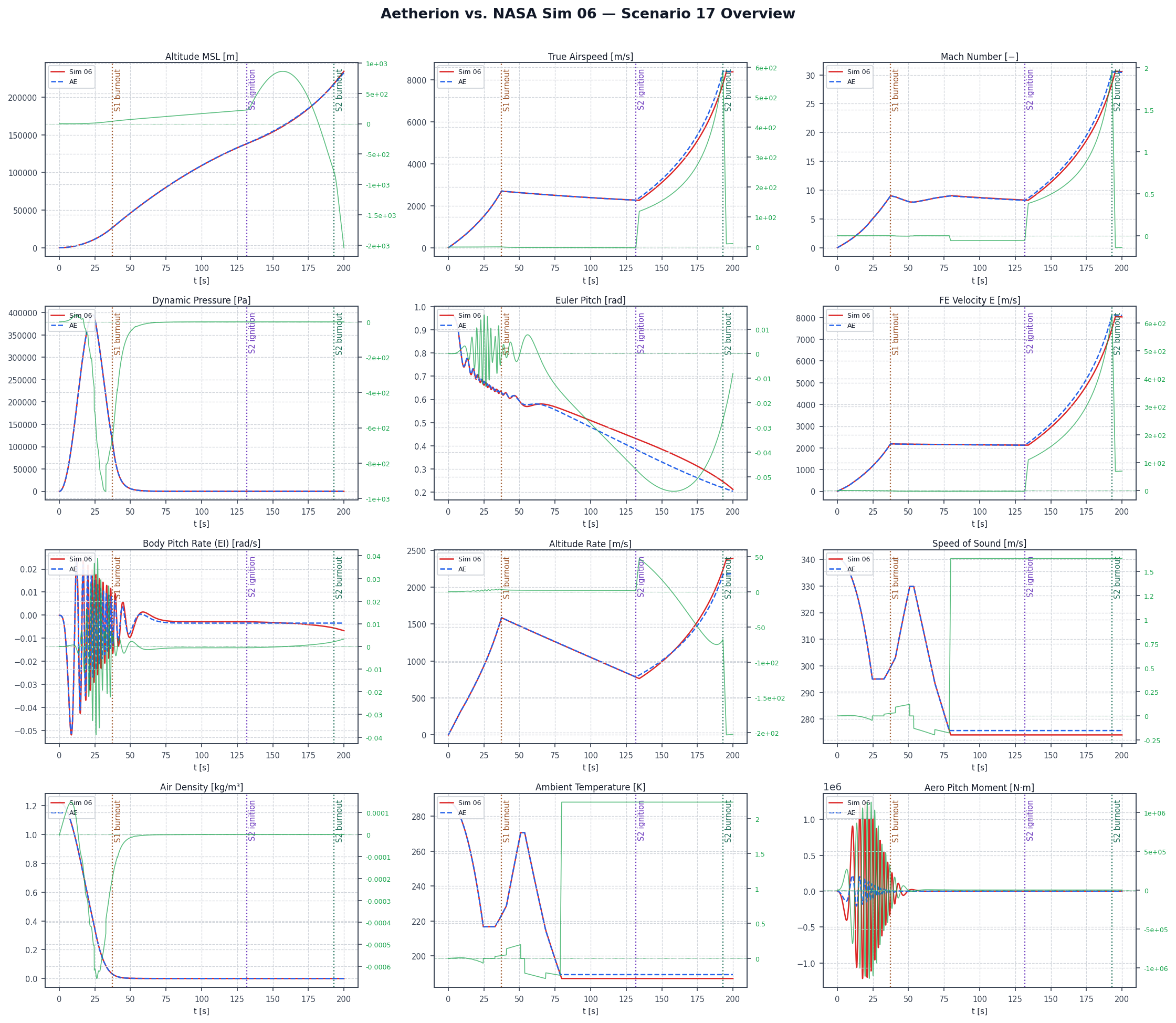
Side-by-side comparison of Aetherion vs. NASA Sim 06 for all key output quantities over the 200-second two-stage ascent.
Altitude — \(h(t)\) with phase markers (final 247.7 km; Sim 04 251.5 km, Sim 06 234.5 km):
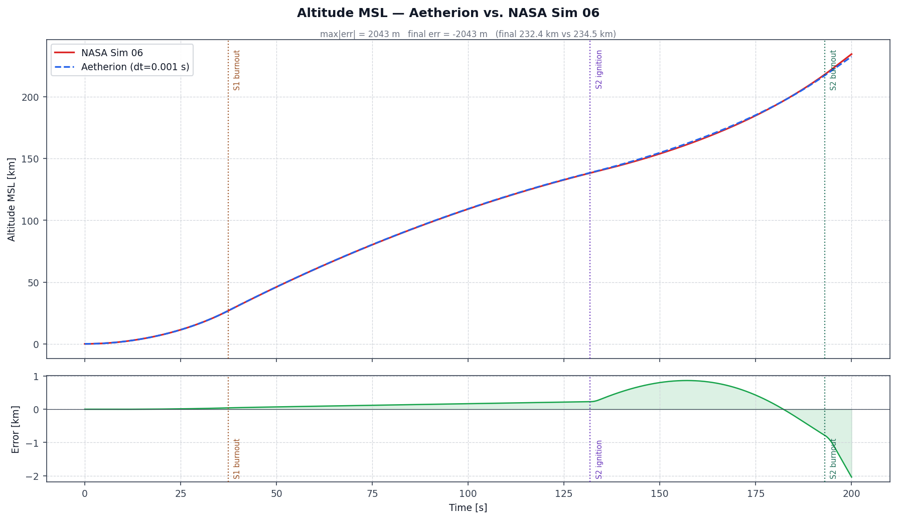
Euler pitch angle — gravity-turn nose-down rotation (final 19.0°; Sim 04 22.3°, Sim 06 12.2°):
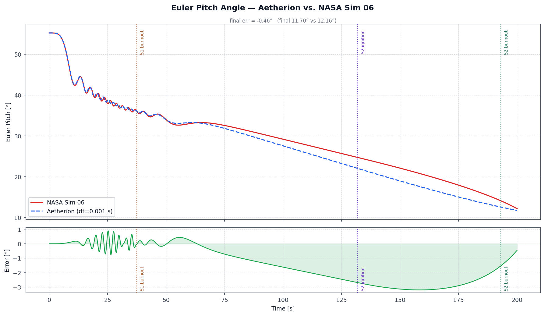
True airspeed — atmosphere-relative speed (final 8 363 m/s; Sim 04 8 336 m/s, Sim 06 8 381 m/s):
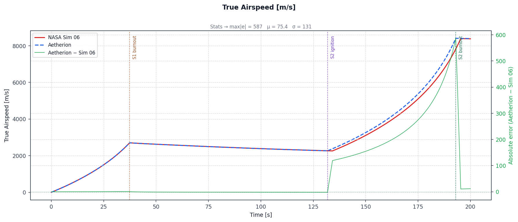
Mach number and dynamic pressure — show S1 max-q and the high-altitude near-vacuum regime after ~80 km:
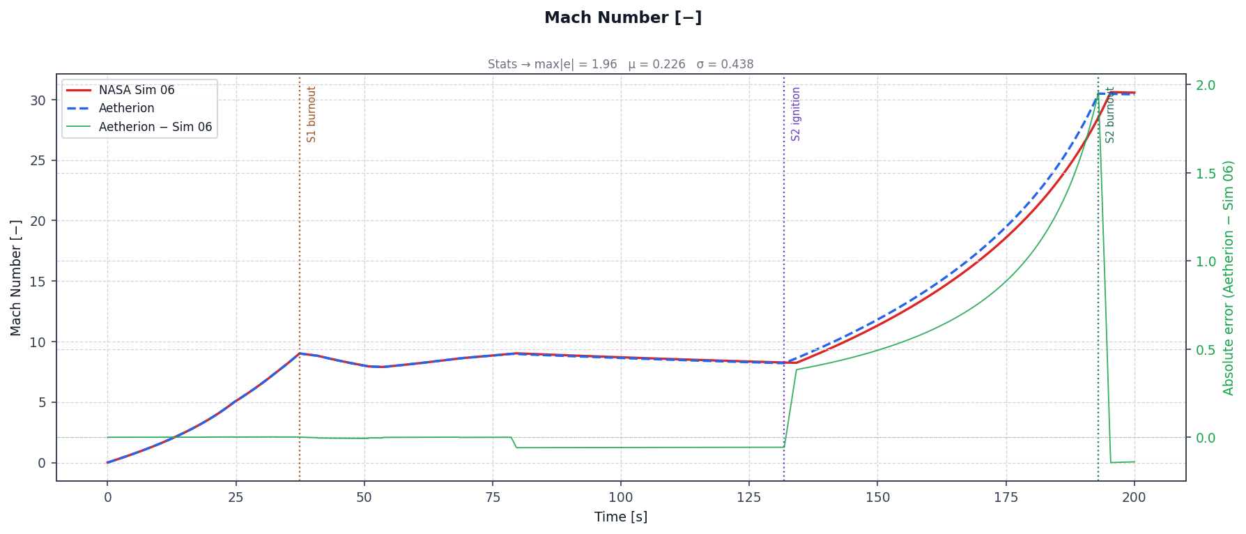
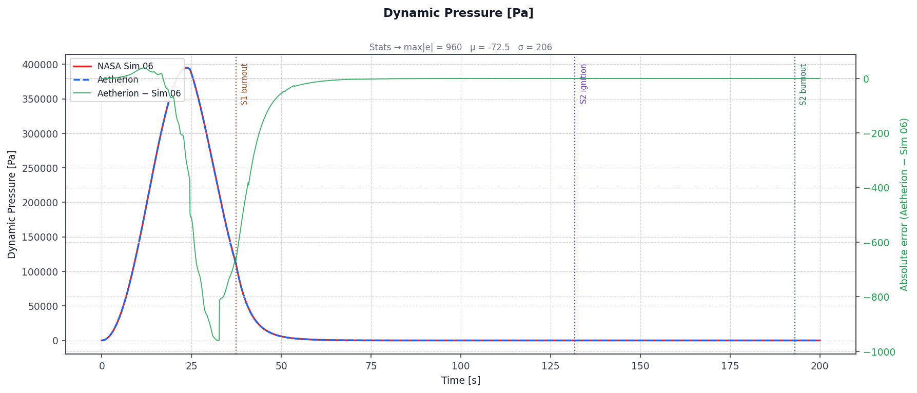
Earth-relative velocity components (NED East is the dominant component for this equatorial, eastward launch):
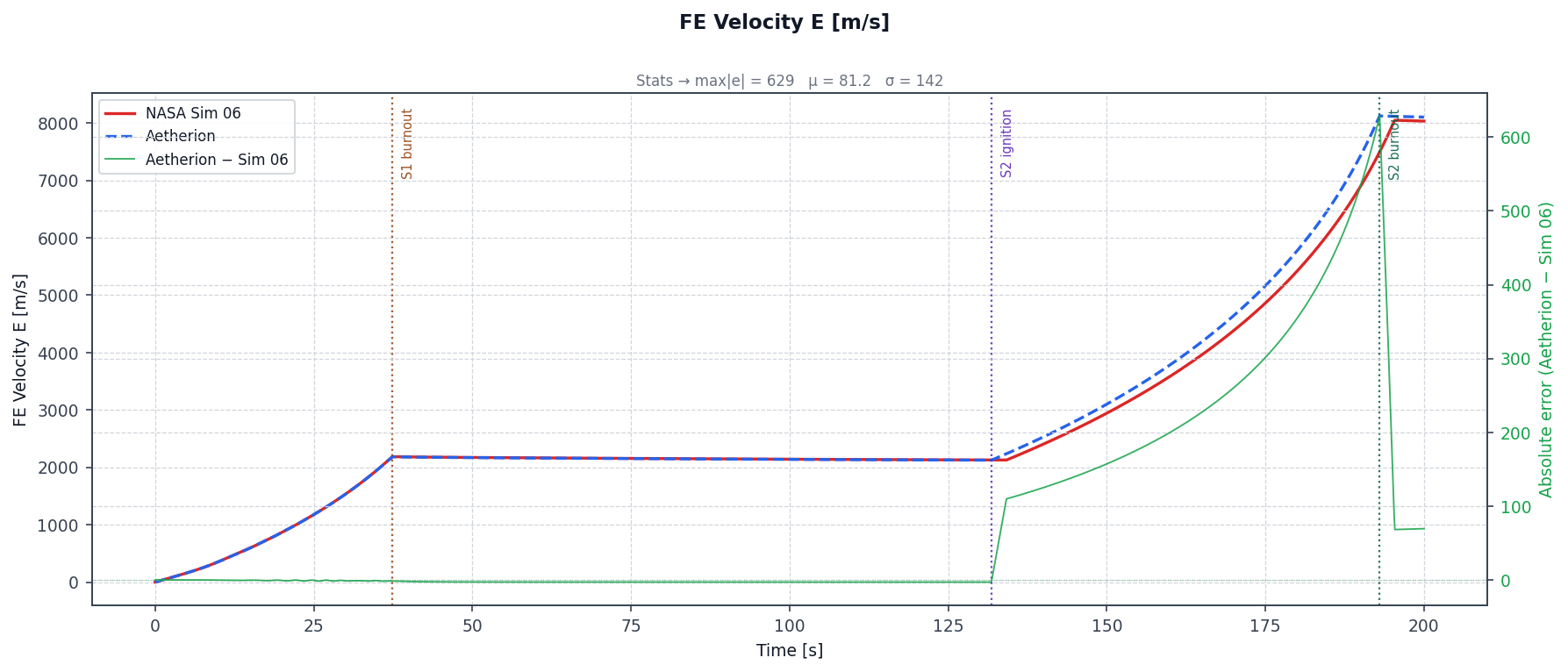
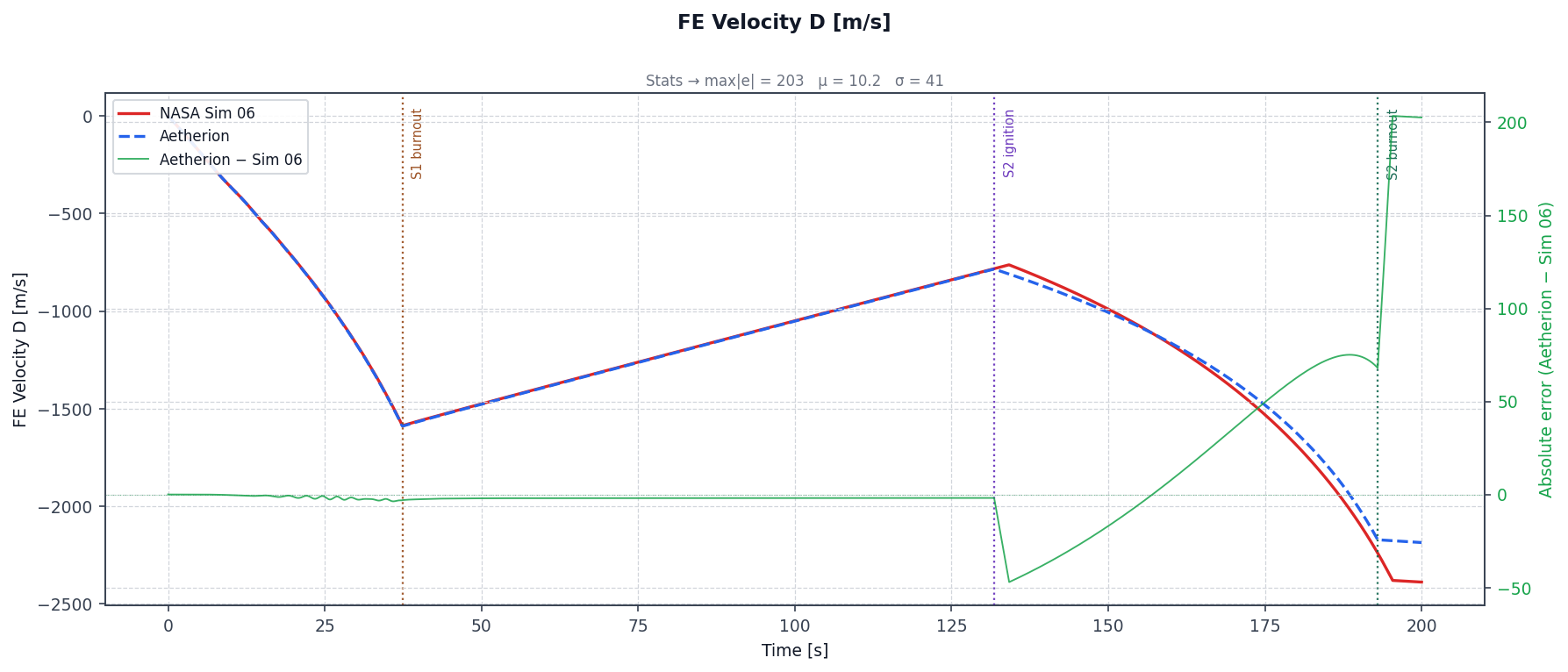
Altitude rate — upward velocity shows S1 and S2 powered ascent clearly:
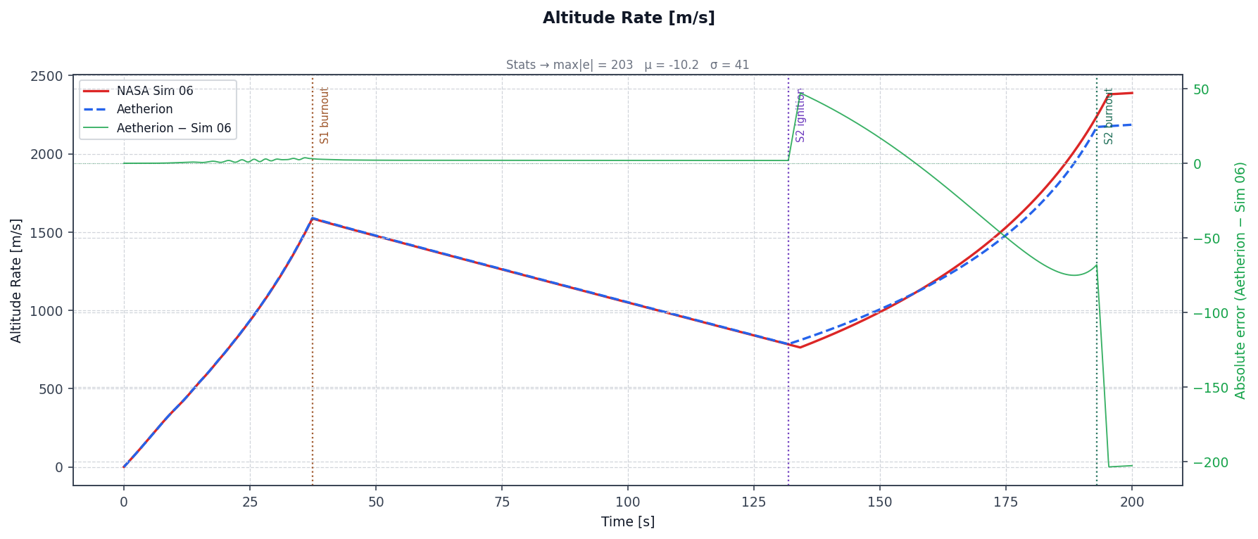
Body pitch rate (ECI-relative) — shows gravity-turn weathervaning and the coast-phase decay:
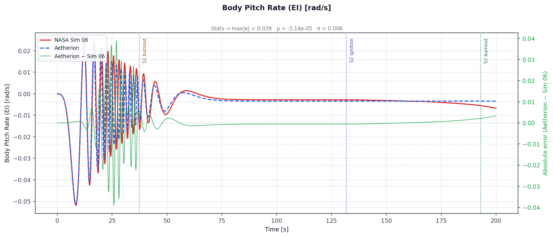
Aerodynamic pitching moment — large during S1 max-q, decays to near-zero above ~70 km:
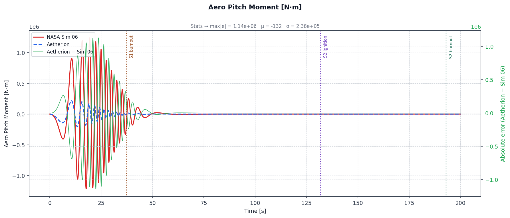
Atmospheric state (US Standard Atmosphere 1976 — the model reaches its 84.852 km ceiling during the coast and applies exponential decay above it):
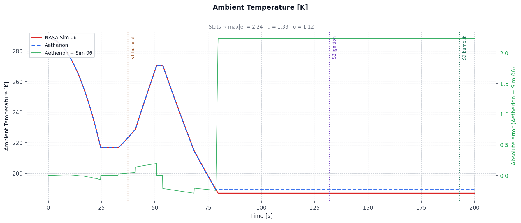
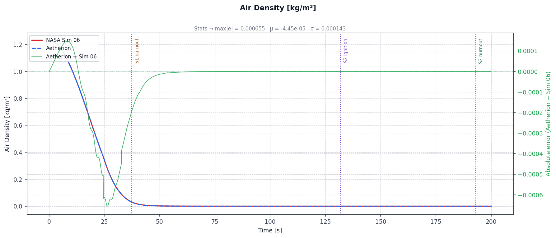
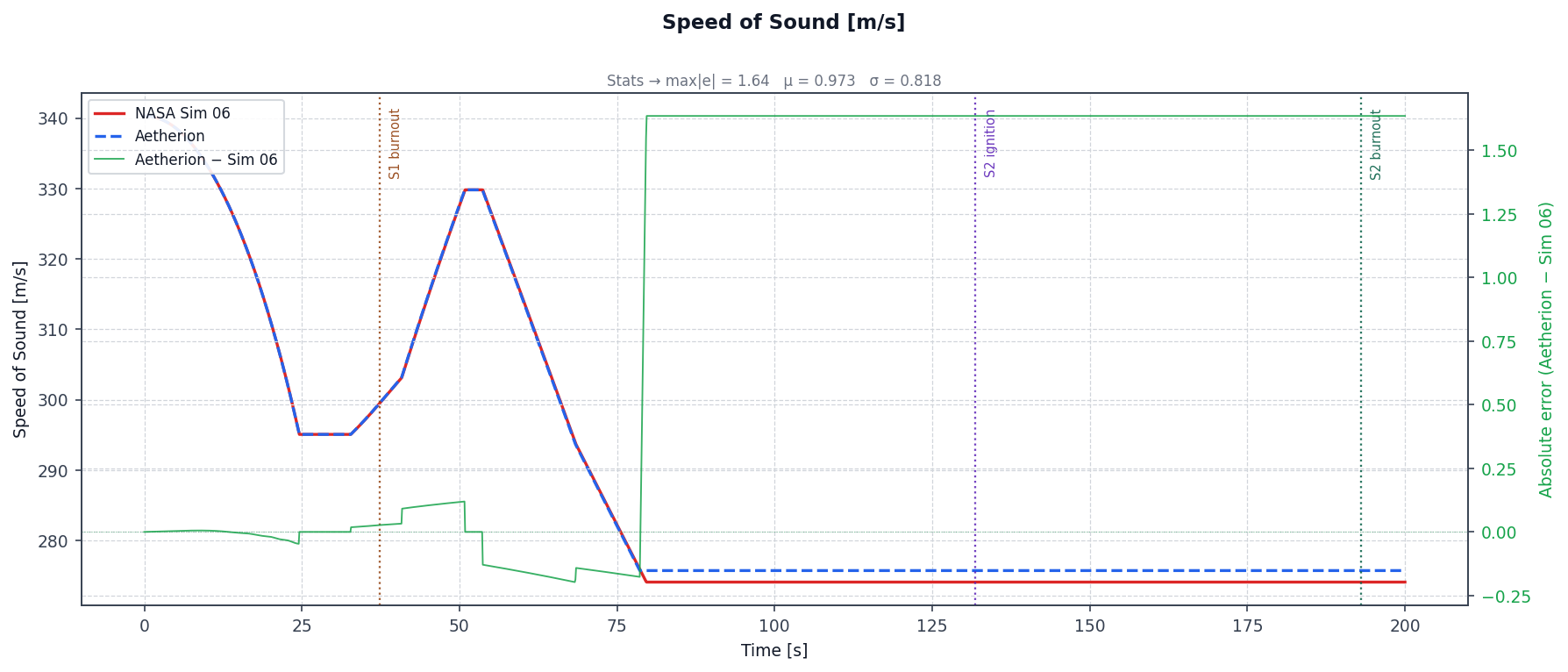
Local gravitational acceleration (J₂ model):
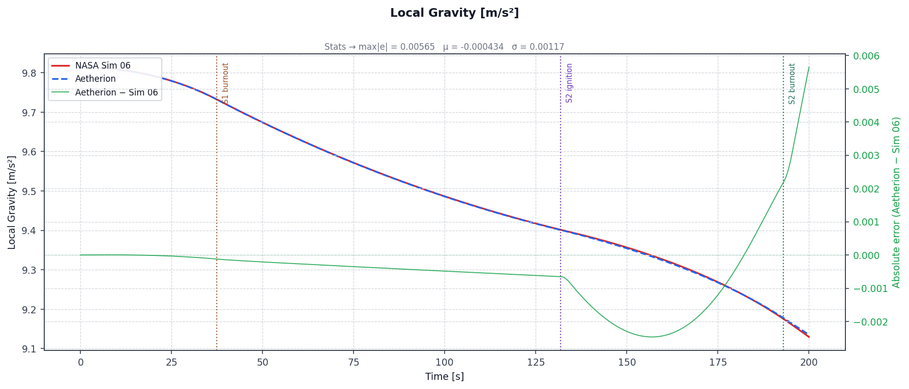
3-D trajectory — East–Up projection from the equatorial launch site. Trajectory segments are colour-coded by mission phase (S1 burn red, ballistic coast blue, S2 burn purple, final coast green). The dashed grey line is NASA Sim 06 and the dash-dot amber line NASA Sim 04. Mission events are annotated with vertical drop lines to the ground plane:
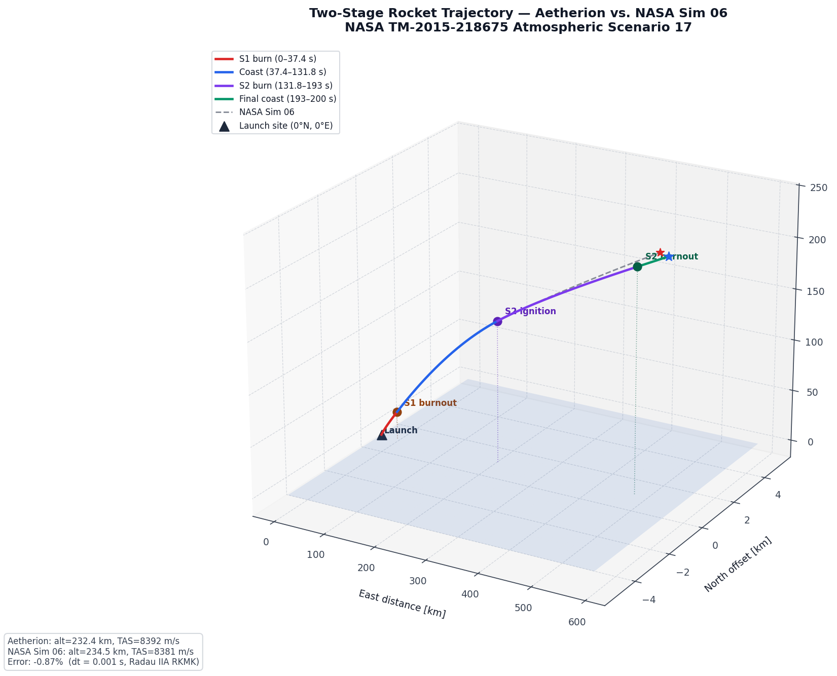
3-D trajectory of the two-stage rocket. The ground plane (altitude = 0) is shown as a translucent blue surface. Phase boundaries at S1 burnout (t = 37.4 s), S2 ignition (t = 131.8 s), and S2 burnout (t = 193 s) are marked with annotated drop-lines. Aetherion ends at 248 km, between the two NASA implementations (Sim 04: 251 km, Sim 06: 234 km), at a speed within 0.4 % of both (8 363 vs 8 336 and 8 381 m/s).
The NASA TM bundle contains three independent reference runs of Scenario 17, all produced by the original check-case code but with different step sizes:
Atmos_17_sim_04.csv— sampled at 0.01 s (no true-airspeed column)Atmos_17_sim_05.csv— sampled at 0.01 sAtmos_17_sim_06.csv— sampled at 0.1 s
The three runs agree closely through the first-stage burn and coast, but diverge sharply after S2 ignition: at \(t = 200\ \text{s}\) sims 04/05 end 17 km above sim_06 with a 10.6° pitch difference. The reference envelope for this scenario is therefore about 1.7 × 10⁴ m wide — an order of magnitude wider than Aetherion’s deviation from the closest run.
Aetherion at \(\Delta t = 0.001\ \text{s}\) (Radau IIA RKMK) ends at 248 km, between the two implementations. The NASA TM recommends an integration time step of \(\Delta t \leq 0.001\ \text{s}\) for this scenario.
The table below gives Sim 04 and Sim 06 side by side (Sim 05 is the same implementation as Sim 04 at a finer step and agrees with it to 7 m); the prose quotes errors against both. Until v0.17.2 these numbers were quoted against Sim 06 only, and the end state agreed with it to 0.9 % because an inertia error (pre-DOI audit finding F02) cancelled the modelling difference described under *Known Modelling Differences*.
Validation Results
The table below compares Aetherion output against NASA Sim 04 and
NASA Sim 06 (data/Atmos_17_TwoStageRocketToOrbit/).
Run with \(\Delta t = 0.001\ \text{s}\), --writeInterval 100,
--endTime 200.
\(t\) [s] |
AltAetherion [m] |
AltSim 04 [m] |
AltSim 06 [m] |
PitchAeth. [°] |
PitchSim 04 [°] |
PitchSim 06 [°] |
TASAetherion [m/s] |
TASSim 04 [m/s] |
TASSim 06 [m/s] |
|---|---|---|---|---|---|---|---|---|---|
0 |
0.0 |
0.0 |
0.0 |
55.22 |
55.22 |
55.22 |
0.00 |
0.10 |
0.10 |
5 |
448.5 |
449.0 |
449.5 |
54.26 |
54.25 |
54.24 |
242.75 |
242.83 |
242.75 |
10 |
1 828.2 |
1 828.6 |
1 829.3 |
43.42 |
43.27 |
43.24 |
509.87 |
509.95 |
509.85 |
20 |
7 253.9 |
7 249.4 |
7 248.4 |
39.68 |
39.59 |
39.63 |
1 132.76 |
1 132.84 |
1 132.62 |
30 |
16 650.1 |
16 634.2 |
16 628.3 |
37.03 |
36.86 |
36.82 |
1 926.75 |
1 926.78 |
1 926.31 |
37.4 (S1 burnout) |
26 789.2 |
26 759.5 |
26 747.1 |
36.23 |
36.25 |
36.13 |
2 700.80 |
2 700.76 |
2 700.39 |
50 (coast) |
46 100.4 |
46 051.9 |
46 027.1 |
34.29 |
34.28 |
33.97 |
2 624.20 |
2 625.88 |
2 625.50 |
100 (coast) |
109 288.9 |
109 185.3 |
109 110.6 |
29.12 |
30.93 |
29.17 |
2 382.79 |
2 384.98 |
2 384.75 |
131.8 (S2 ignites) |
138 480.7 |
138 345.0 |
138 238.7 |
25.43 |
28.58 |
24.72 |
2 264.59 |
2 267.03 |
2 266.91 |
150 (S2 burn) |
155 232.2 |
154 455.7 |
153 859.6 |
23.38 |
27.21 |
22.08 |
3 254.61 |
3 097.49 |
3 105.22 |
175 (S2 burn) |
189 387.6 |
189 142.4 |
184 730.7 |
20.87 |
25.09 |
17.91 |
5 356.41 |
5 072.55 |
5 098.14 |
200 (end) |
247 711.7 |
251 450.8 |
234 477.0 |
18.96 |
22.26 |
12.16 |
8 363.28 |
8 335.71 |
8 380.79 |
Through the S1 burn phase (t = 0–37.4 s) the altitude difference is below 1.3 m for the first 6.5 s (the altitude itself is still under 770 m there, so a relative error is not yet meaningful) and then within 0.11 % of Sim 04 and 0.16 % of Sim 06 to burnout; the speed stays within 0.1 m/s of Sim 04 and 0.6 m/s of Sim 06. The pitch rate reverses twice during the burn, under the aerodynamic moment, and Aetherion follows Sim 06 through both reversals (e.g. +0.85 °/s against +1.10 °/s at t = 20 s, −0.58 against −0.44 °/s at t = 25 s). Through the coast phase (t = 37.4–131.8 s) the altitude offset stays at 0.10–0.11 % (Sim 04) and 0.16–0.18 % (Sim 06), as it must for ballistic flight, and the pitch at t = 100 s is 29.12° against 29.17° (Sim 06) and 30.93° (Sim 04): the two NASA implementations leave the burn with different pitch rates (−0.097 and −0.163 °/s) and Aetherion’s −0.139 °/s lies between them. At S2 ignition (t = 131.8 s) the altitude is within 0.10 % / 0.18 % and the pitch is 25.4° against 28.6° / 24.7°.
Through the S2 burn the three diverge. Both NASA implementations let the pitch rate grow as the stage empties (to −0.20 and −0.39 °/s at t = 200 s), while Aetherion’s stays constant (see Known Modelling Differences), and the NASA runs end 17 km and 10° apart from each other. The final state at t = 200 s:
Altitude: 247.7 km — −1.5 % against Sim 04 (251.5 km), +5.6 % against Sim 06 (234.5 km); between the two.
TAS: 8 363 m/s — +0.33 % against Sim 04 (8 336 m/s), −0.21 % against Sim 06 (8 381 m/s).
Pitch: 18.96° — −3.3° against Sim 04 (22.26°), +6.8° against Sim 06 (12.16°); between the two.
Known Modelling Differences
Item |
Explanation |
|---|---|
Angular momentum of a burning stage |
The spatial inertia is rebuilt before every step (zero-order hold) and the body rate \(\boldsymbol{\omega}\) is kept through the rebuild, so the pitch rate stays constant in vacuum. The NASA reference runs do something else, and not the same thing as each other: through the S2 burn, over which \(I_{yy}\) falls by a factor 4.4, the pitch rate of Sims 04/05 grows 2.1-fold (−0.10 to −0.20 °/s) and that of Sim 06 2.4-fold (−0.16 to −0.39 °/s). The complete variable-mass equation (Thomson) is \(\mathbf{I}\dot{\boldsymbol{\omega}} = \mathbf{M}_\text{ext} - \dot{\mathbf{I}}\boldsymbol{\omega} - \dot{m}\,\rho_e^2\,\boldsymbol{\omega}\): the inertia-relief term \(-\dot{\mathbf{I}}\boldsymbol{\omega}\) raises the rate as the tensor shrinks, and the jet-damping term lowers it, with \(\rho_e\) the nozzle’s distance from the centre of mass. Keeping \(\boldsymbol{\omega}\) is the case \(\rho_e = k\), the propellant’s radius of gyration about the centre of mass – the propellant leaves with the angular momentum it had where it sat; the DML gives \(k^2 = \Delta I/\Delta m = 9.1\ \text{m}^2\), \(k \approx 3\ \text{m}\). Relief alone (\(\rho_e = 0\), i.e. conserving \(\mathbf{I}_C\boldsymbol{\omega}\)) would raise the rate 4.4-fold; it was tried and ends at 3.4° of pitch, outside the reference spread. A real second stage has its nozzle well beyond \(k\) (here some 5–6 m behind the centre of mass), so jet damping outweighs relief and the pitch rate should fall through the burn, with a time constant \(I/(\dot m \rho_e^2)\) of order 10 s. The DML does not give the nozzle position, so that term is not modelled; the reference runs do not model it either, and their growth is a convention of how their codes handle \(\dot{\mathbf{I}}\), not an effect that can be derived from the vehicle data. Keeping \(\boldsymbol{\omega}\) is therefore retained as the closer of the two available limits to the physics. This is the largest contributor to the end-state spread, both between Aetherion and the references and among the references themselves (see below). |